Build a Large Language Model (From Scratch)
GitHub(相关代码): https://github.com/rasbt/LLMs-from-scratch
【其他参考】The Illustrated Transformer(图的形式讲解transformer,涉及到本书要讲的qkv计算、多head注意力等): https://jalammar.github.io/illustrated-transformer/
- 【其他代码】实现了类似功能: https://github.com/jingyaogong/minimind
1. Understanding LLM
章节:
1.1 What is an LLM?
1.2 Applications of LLMs
1.3 Stages of building and using LLMs
1.4 Using LLMs for different tasks
1.5 Utilizing large datasets
1.6 A closer look at the GPT architecture
1.7 Building a large language model
1.8 Summary
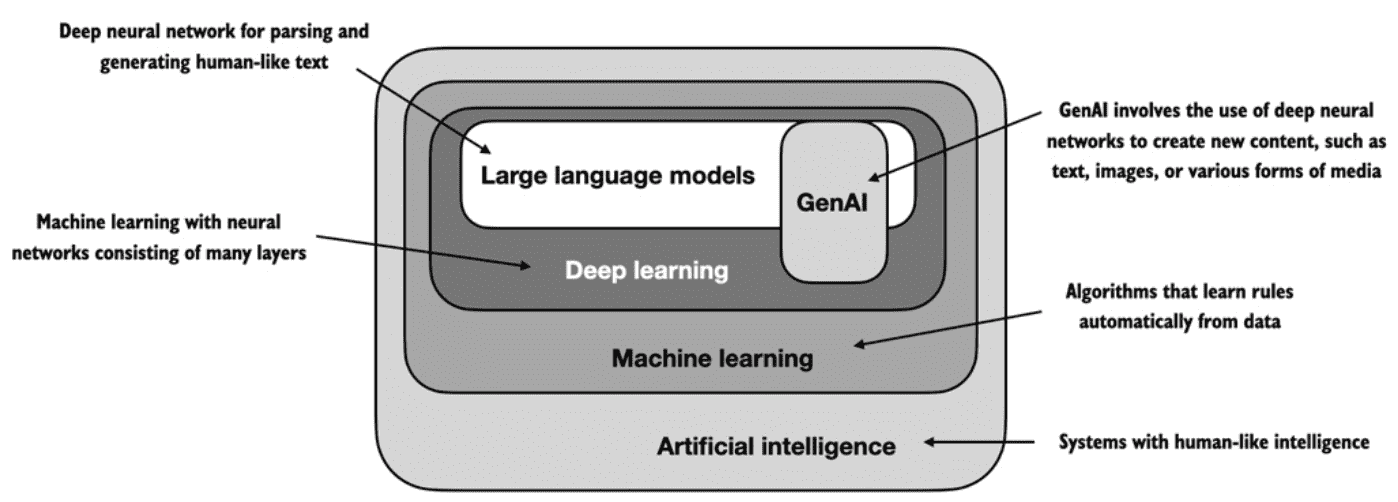
AI including:
machine learning
deep learning

rule-based systems
genetic algorithms
expert systems
fuzzy logic
symbolic reasoning
traditional machine learning: human experts might manually extract features from email text such as the frequency of certain trigger words (“prize,” “win,” “free”), the number of exclamation marks, use of all uppercase words, or the presence of suspicious links.
deep learning: does not require manual feature extraction. This means that human experts do not need to identify and select the most relevant features for a deep learning model.
备注
不管是traditional machine learning还是deep learning,都需要人工收集一些数据,哪此邮件是spam,哪些不是spam。但 traditional machine learning 还需要专家进行人工的特征提取,对垃圾邮件事例特征有:win, free单词很多,有可疑链接,使用大写字母……
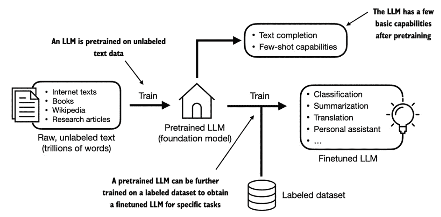
Figure 1.3
The two most popular categories of finetuning LLMs:
1. instruction-finetuning
2. finetuning for classification tasks
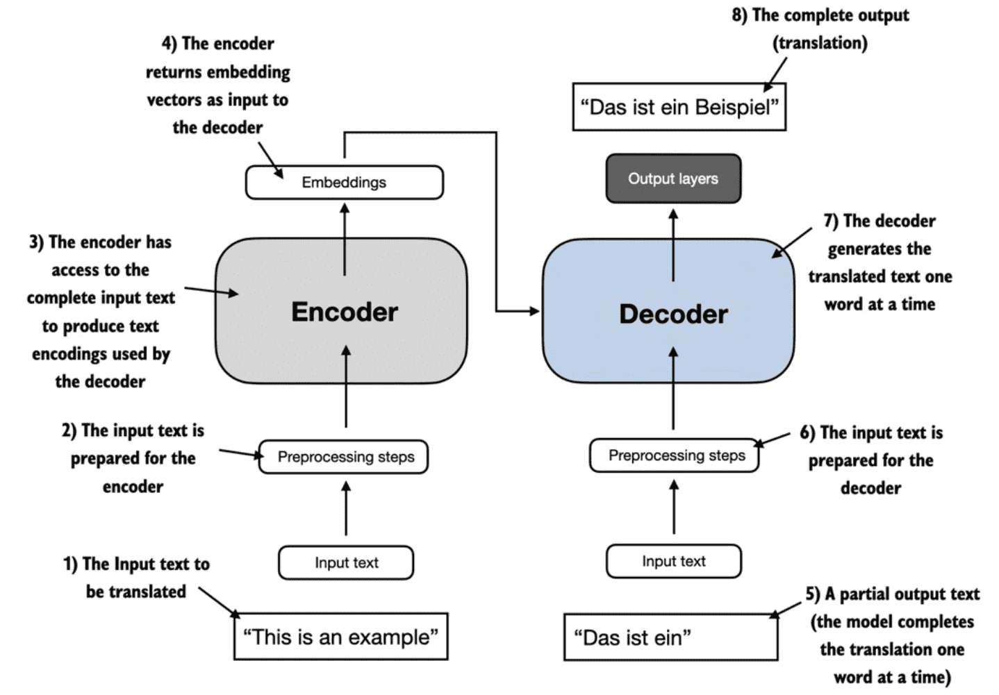
Figure 1.4 A simplified depiction of the original transformer architecture, which is a deep learning model for language translation. The transformer consists of two parts, an encoder that processes the input text and produces an embedding representation (a numerical representation that captures many different factors in different dimensions) of the text that the decoder can use to generate the translated text one word at a time. Note that this figure shows the final stage of the translation process where the decoder has to generate only the final word (“Beispiel”), given the original input text (“This is an example”) and a partially translated sentence (“Das ist ein”), to complete the translation.
A key component of transformers and LLMs is the self-attention mechanism, which allows the model to weigh the importance of different words or tokens in a sequence relative to each other.
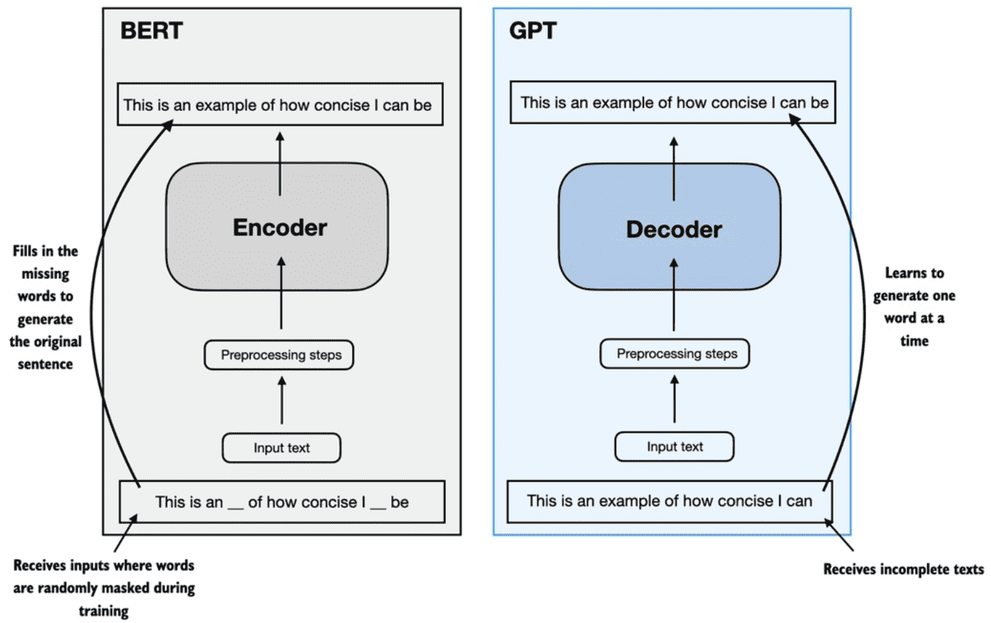
Figure 1.5 A visual representation of the transformer’s encoder and decoder submodules. On the left, the encoder segment exemplifies BERT-like LLMs, which focus on masked word prediction and are primarily used for tasks like text classification. On the right, the decoder segment showcases GPT-like LLMs, designed for generative tasks and producing coherent text sequences.
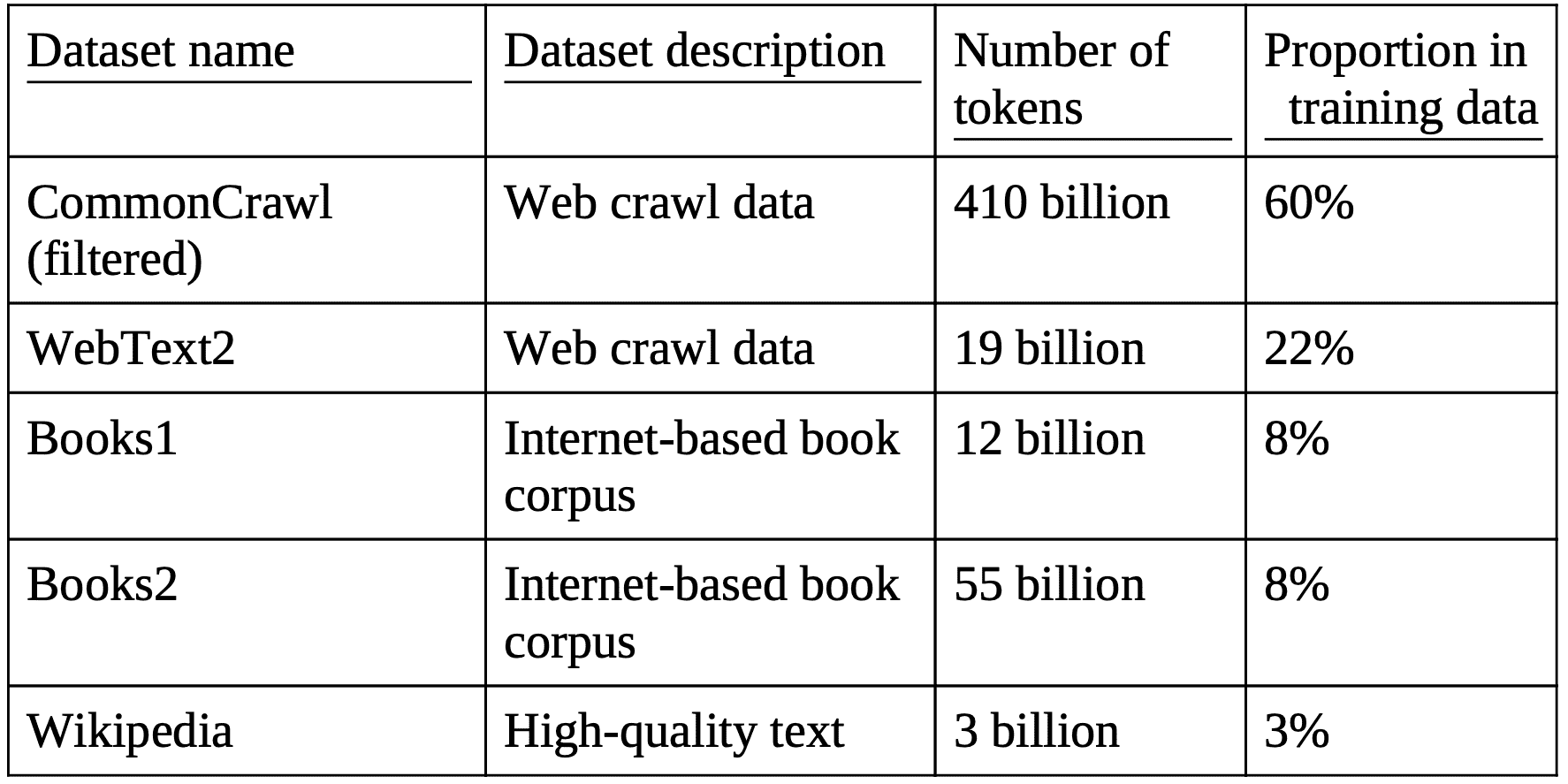
Table 1.1 The pretraining dataset of the popular GPT-3 LLM
* Wikipedia corpus consists of English-language Wikipedia
* Books1 is likely a sample from Project Gutenberg: https://www.gutenberg.org/
* Books2 is likely from Libgen: https://en.wikipedia.org/wiki/Library_Genesis
* CommonCrawl is a filtered subset of the CommonCrawl database: https://commoncrawl.org/
* WebText2 is the text of web pages from all outbound Reddit links from posts with 3+ upvotes.
The ability to perform tasks that the model wasn’t explicitly trained to perform is called an “emergent behavior(涌现行为).”“涌现行为” 指的是模型在规模增大后自发展现出一些未明确训练的能力(如推理、算术等),这些能力不是直接由个体参数或特定任务驱动的,而是系统在规模和复杂度增加时的自发产物。
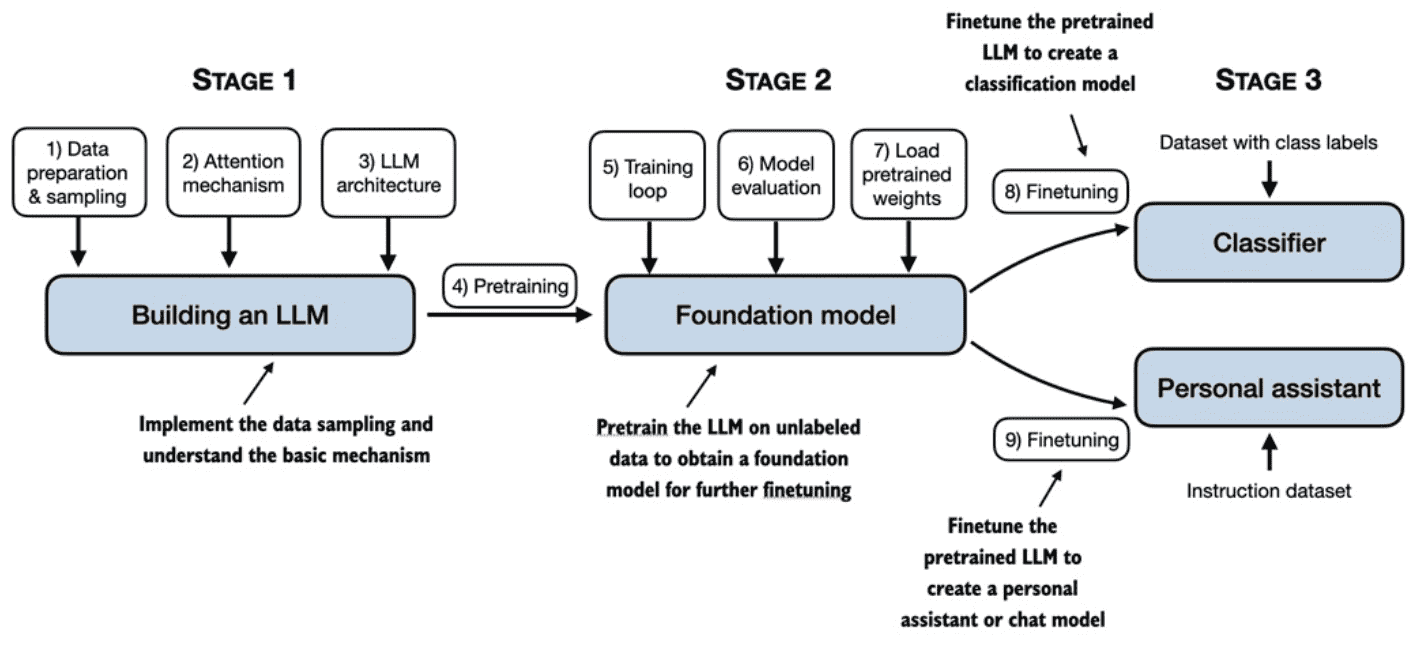
Figure 1.9 The stages of building LLMs covered in this book include implementing the LLM architecture and data preparation process, pretraining an LLM to create a foundation model, and finetuning the foundation model to become a personal assistant or text classifier.
2. Working with Text Data
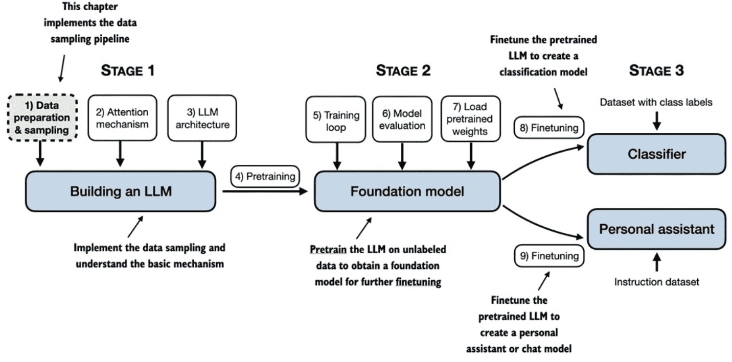
Figure 2.1 A mental model of the three main stages of coding an LLM, pretraining the LLM on a general text dataset, and finetuning it on a labeled dataset. This chapter will explain and code the data preparation and sampling pipeline that provides the LLM with the text data for pretraining.
2.1 Understanding word embeddings
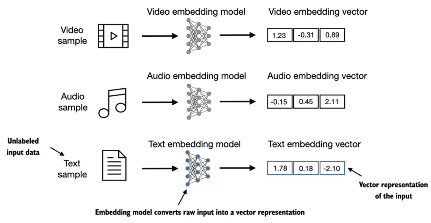
Figure 2.2 Deep learning models cannot process data formats like video, audio, and text in their raw form. Thus, we use an embedding model to transform this raw data into a dense vector representation that deep learning architectures can easily understand and process. Specifically, this figure illustrates the process of converting raw data into a three-dimensional numerical vector.
While word embeddings are the most common form of text embedding, there are also embeddings for sentences, paragraphs, or whole documents. Sentence or paragraph embeddings are popular choices for retrieval- augmented generation.
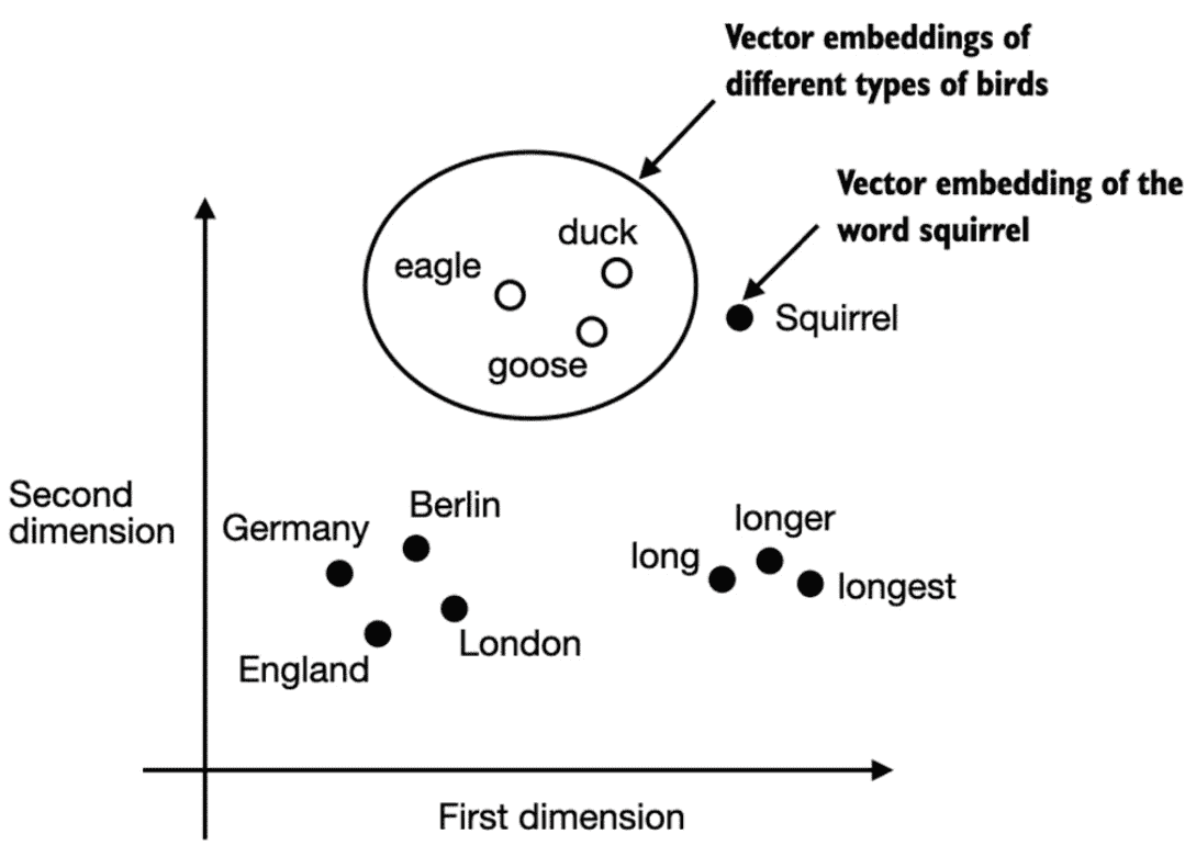
Figure 2.3 If word embeddings are two-dimensional, we can plot them in a two-dimensional scatterplot for visualization purposes as shown here. When using word embedding techniques, such as Word2Vec, words corresponding to similar concepts often appear close to each other in the embedding space. For instance, different types of birds appear closer to each other in the embedding space compared to countries and cities.
Word embeddings can have varying dimensions, from one to thousands. As shown in Figure 2.3, we can choose two-dimensional word embeddings for visualization purposes.
2.2 Tokenizing text
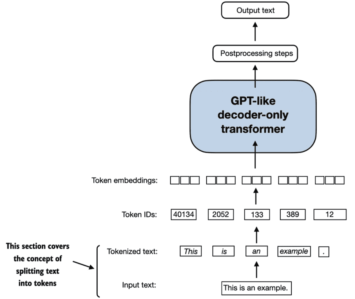
Figure 2.4 A view of the text processing steps covered in this section in the context of an LLM. Here, we split an input text into individual tokens, which are either words or special characters, such as punctuation characters. In upcoming sections, we will convert the text into token IDs and create token embeddings.
2.3 Converting tokens into token IDs
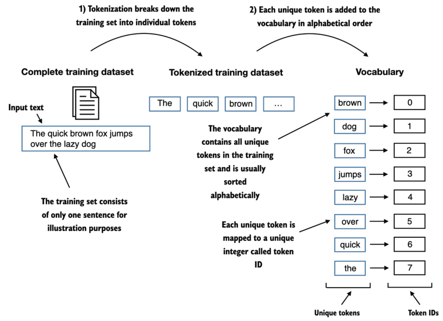
Figure 2.6 We build a vocabulary by tokenizing the entire text in a training dataset into individual tokens. These individual tokens are then sorted alphabetically, and duplicate tokens are removed. The unique tokens are then aggregated into a vocabulary that defines a mapping from each unique token to a unique integer value. The depicted vocabulary is purposefully small for illustration purposes and contains no punctuation or special characters for simplicity.
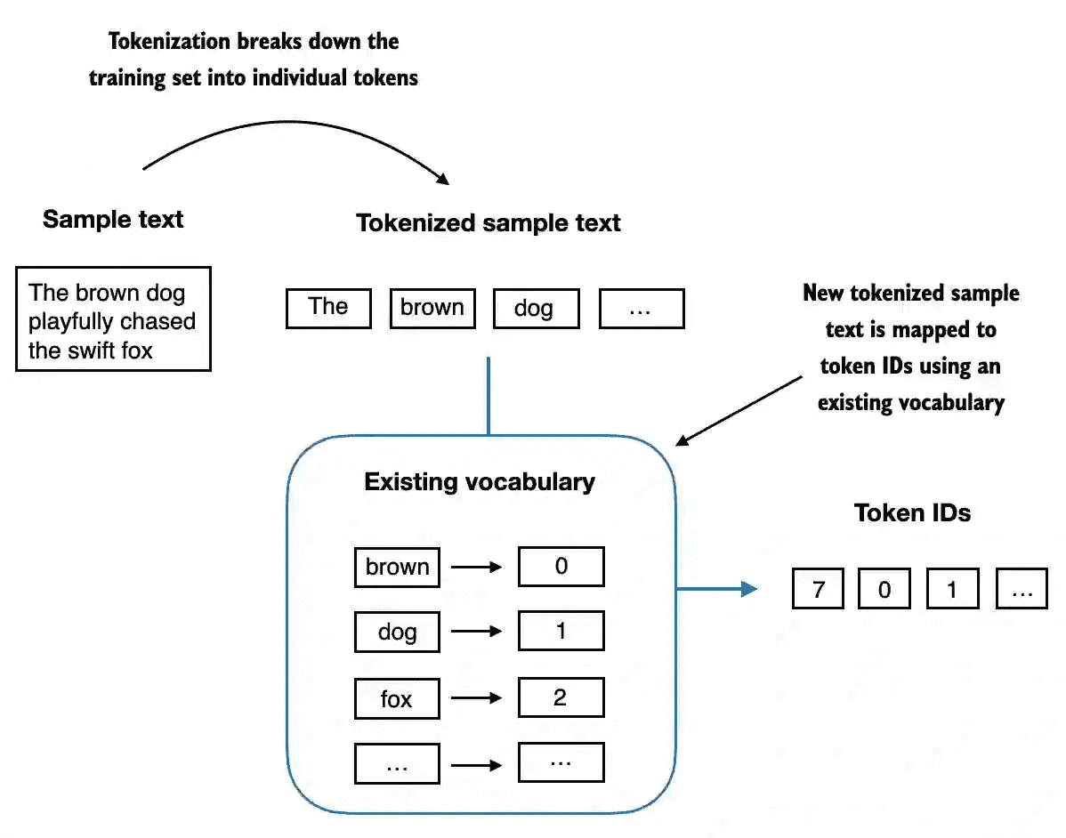
Figure 2.7 Starting with a new text sample, we tokenize the text and use the vocabulary to convert the text tokens into token IDs. The vocabulary is built from the entire training set and can be applied to the training set itself and any new text samples. The depicted vocabulary contains no punctuation or special characters for simplicity.
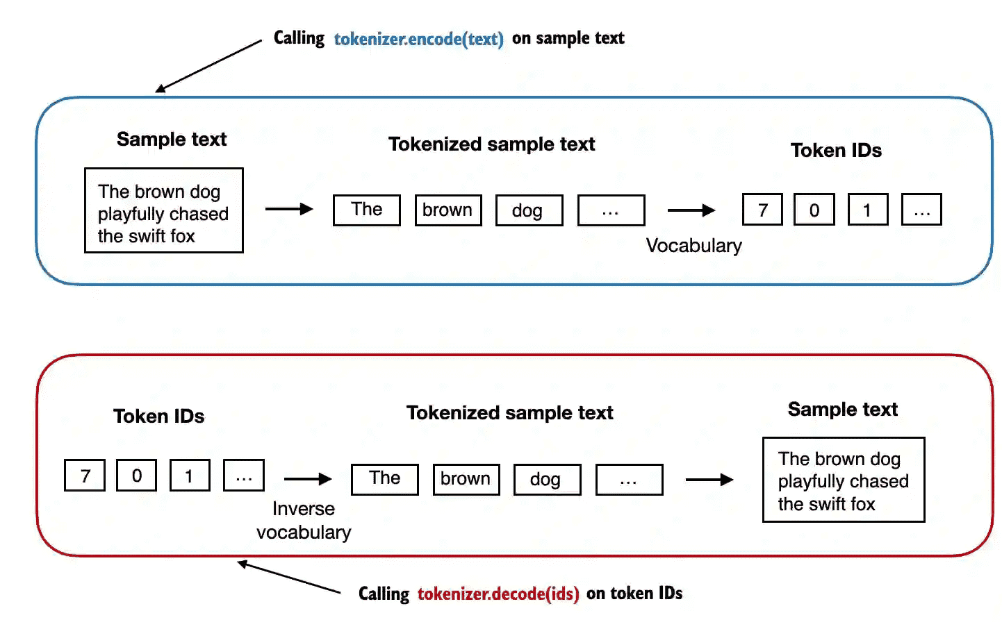
Figure 2.8 Tokenizer implementations share two common methods: an encode method and a decode method. The encode method takes in the sample text, splits it into individual tokens, and converts the tokens into token IDs via the vocabulary. The decode method takes in token IDs, converts them back into text tokens, and concatenates the text tokens into natural text.
2.4 Adding special context tokens
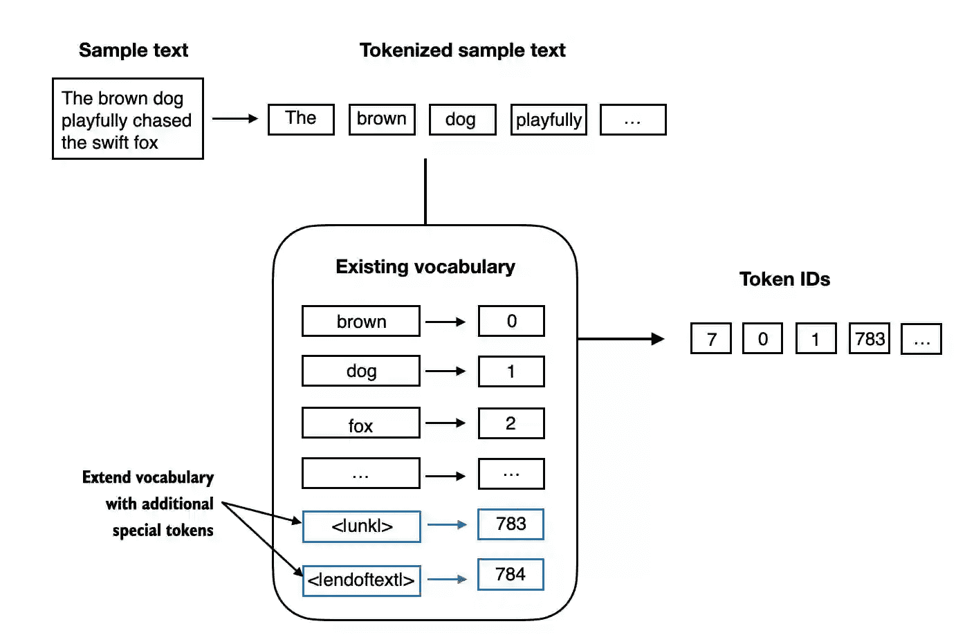
Figure 2.9 We add special tokens to a vocabulary to deal with certain contexts. For instance, we add an <|unk|> token to represent new and unknown words that were not part of the training data and thus not part of the existing vocabulary. Furthermore, we add an <|endoftext|> token that we can use to separate two unrelated text sources.
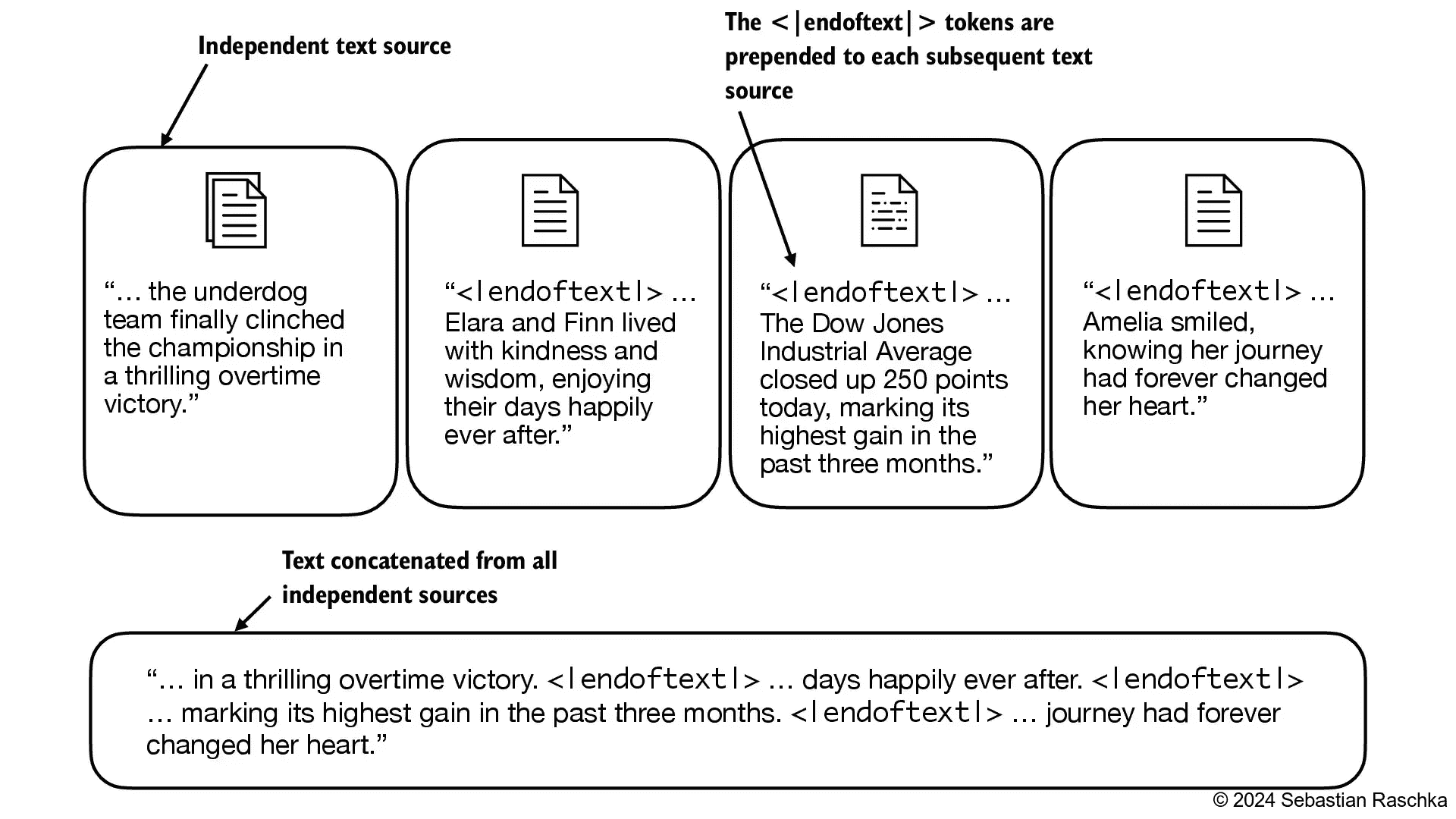
Figure 2.10 When working with multiple independent text source, we add <|endoftext|> tokens between these texts. These <|endoftext|> tokens act as markers, signaling the start or end of a particular segment, allowing for more effective processing and understanding by the LLM.
additional special tokens:
1. [BOS] (beginning of sequence)
2. [EOS] (end of sequence)
3. [PAD] (padding)
4. |endoftext|
5. |unk|
2.5 Byte pair encoding
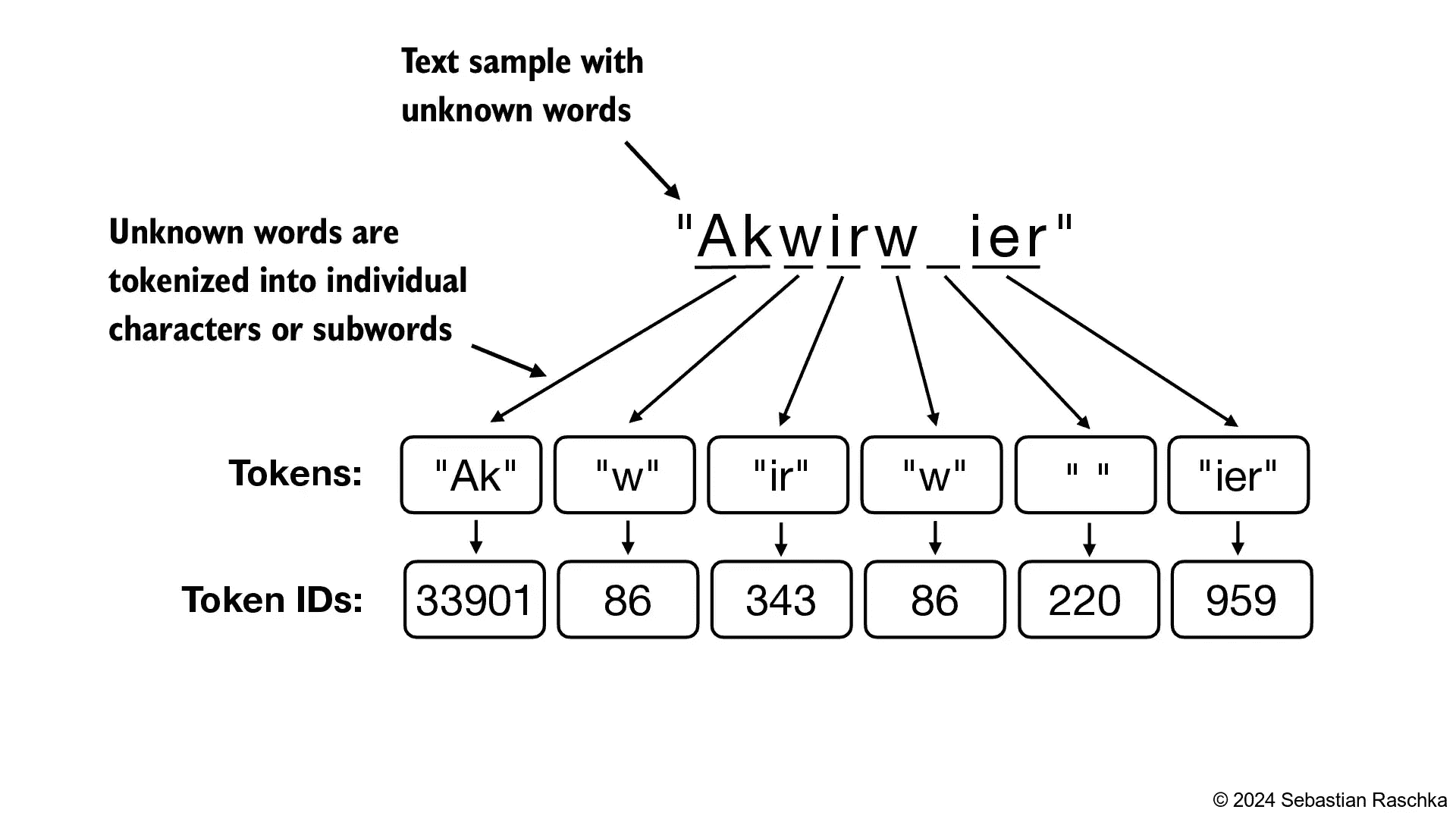
Figure 2.11 BPE tokenizers break down unknown words into subwords and individual characters. This way, a BPE tokenizer can parse any word and doesn’t need to replace unknown words with special tokens, such as <|unk|>.
The original BPE tokenizer can be found here: [https://github.com/openai/gpt-2/blob/master/src/encoder.py](https://github.com/openai/gpt-2/blob/master/src/encoder.py)
The BPE tokenizer from OpenAI’s open-source [tiktoken](https://github.com/openai/tiktoken) library, which implements its core algorithms in Rust to improve computational performance
2.6 Data sampling with a sliding window
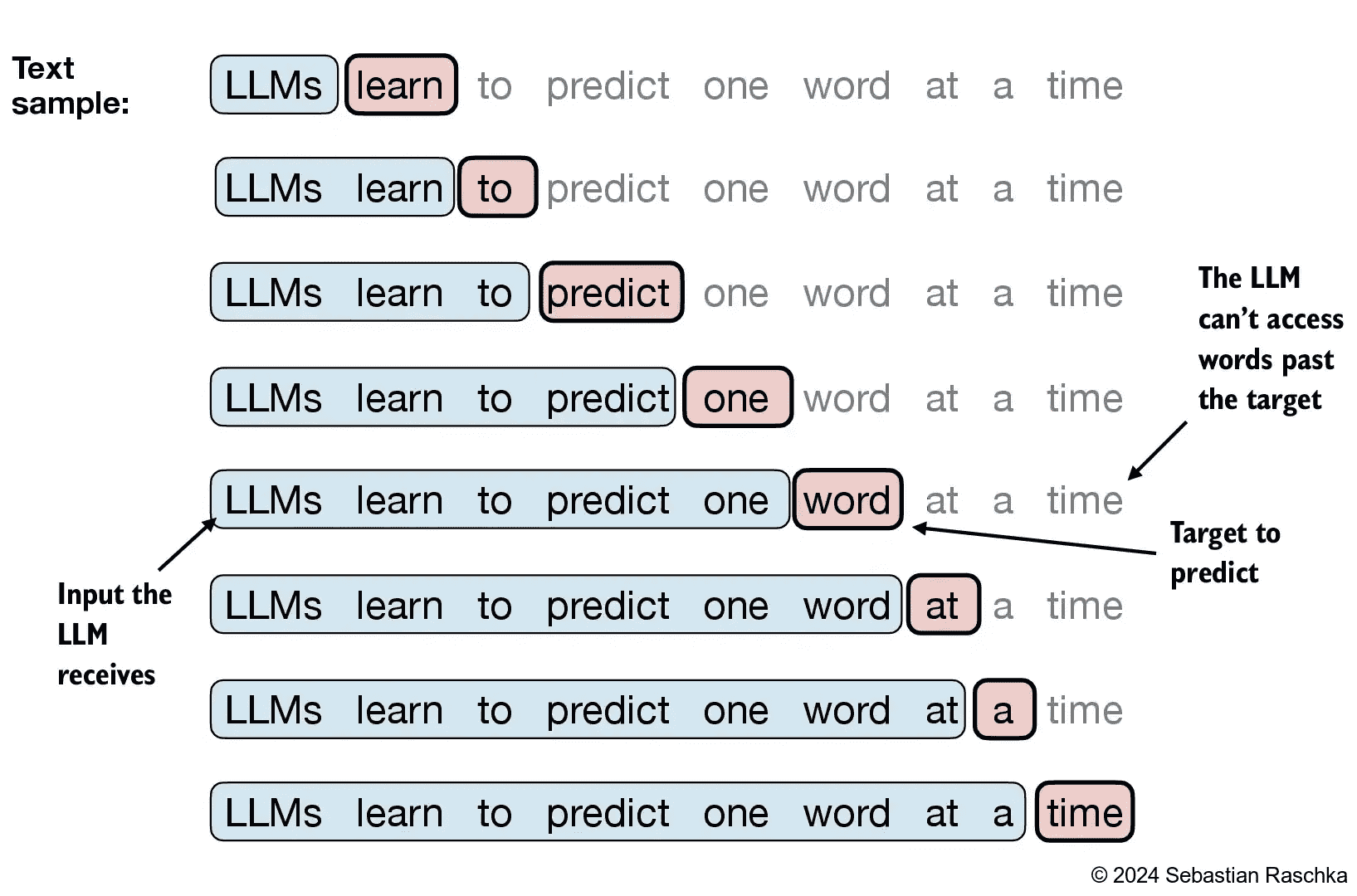
Figure 2.12 Given a text sample, extract input blocks as subsamples that serve as input to the LLM, and the LLM’s prediction task during training is to predict the next word that follows the input block. During training, we mask out all words that are past the target. Note that the text shown in this figure would undergo tokenization before the LLM can process it; however, this figure omits the tokenization step for clarity.
For each text chunk, we want the inputs and targets
Since we want the model to predict the next word, the targets are the inputs shifted by one position to the right
The prediction would look like as follows:(input-target pairs):
and ---->  established
and established ---->  himself
and established himself ---->  in
and established himself in ---->  a
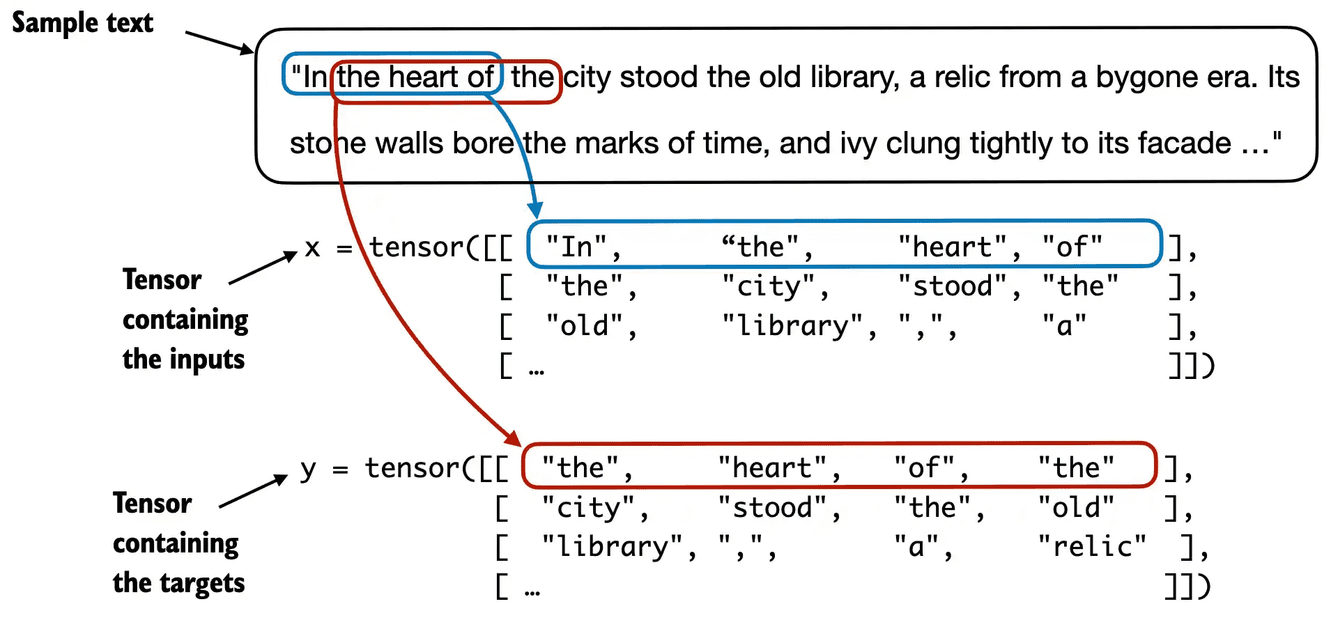
Figure 2.13 To implement efficient data loaders, we collect the inputs in a tensor, x, where each row represents one input context. A second tensor, y, contains the corresponding prediction targets (next words), which are created by shifting the input by one position.
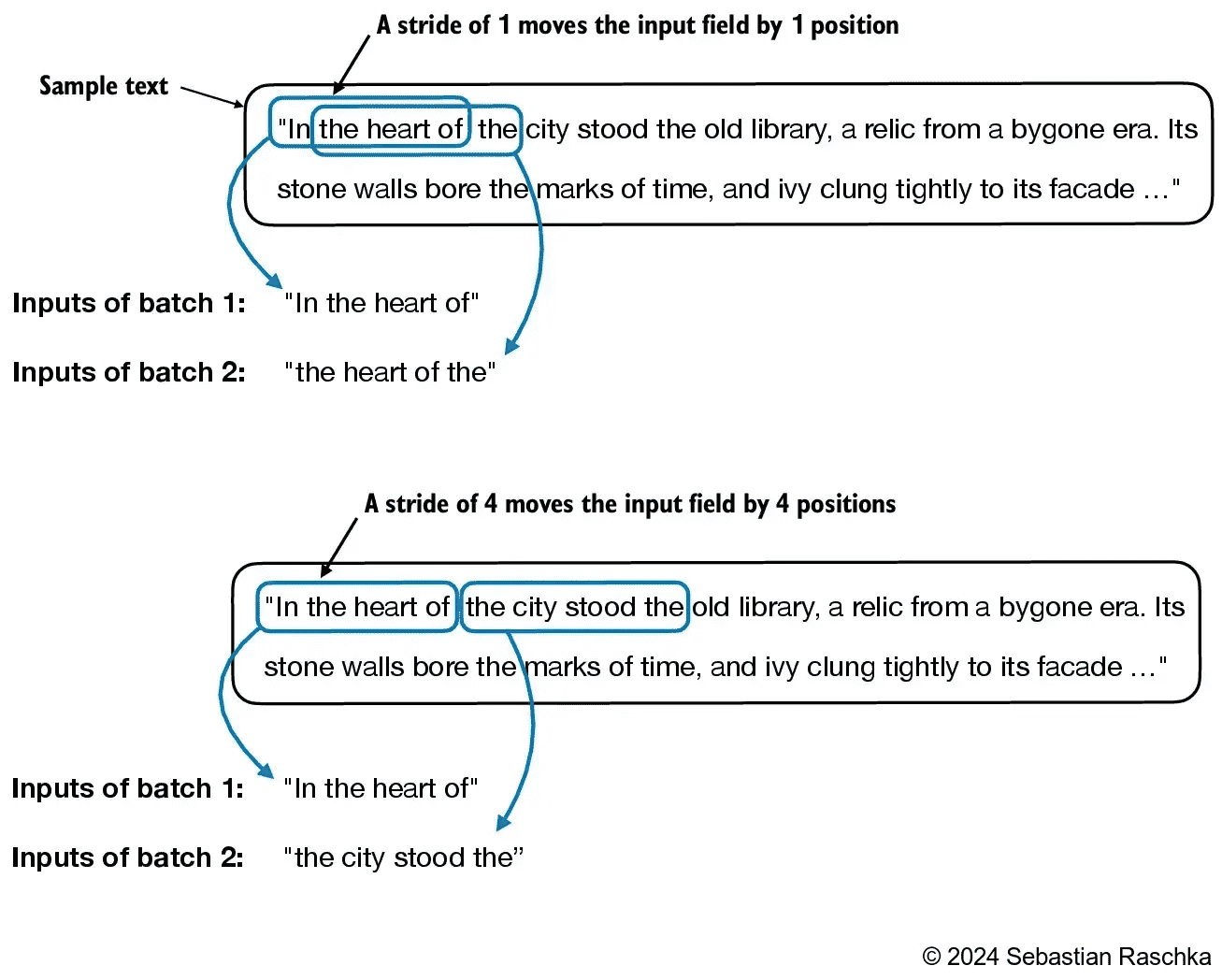
Figure 2.14 When creating multiple batches from the input dataset, we slide an input window across the text. If the stride is set to 1, we shift the input window by 1 position when creating the next batch. If we set the stride equal to the input window size, we can prevent overlaps between the batches.
Small batch sizes require less memory during training but lead to more noisy model updates. The batch size is a trade-off and hyperparameter to experiment with when training LLMs.
示例(batch_size=1, max_length=4, stride=1):
[tensor([[ 40, 367, 2885, 1464]]), tensor([[ 367, 2885, 1464, 1807]])]
示例(batch_size=8, max_length=4, stride=4):
Inputs:
 tensor([[   40,   367,  2885,  1464],
        [ 1807,  3619,   402,   271],
        [10899,  2138,   257,  7026],
        [15632,   438,  2016,   257],
        [  922,  5891,  1576,   438],
        [  568,   340,   373,   645],
        [ 1049,  5975,   284,   502],
        [  284,  3285,   326,    11]])

Targets:
 tensor([[  367,  2885,  1464,  1807],
        [ 3619,   402,   271, 10899],
        [ 2138,   257,  7026, 15632],
        [  438,  2016,   257,   922],
        [ 5891,  1576,   438,   568],
        [  340,   373,   645,  1049],
        [ 5975,   284,   502,   284],
        [ 3285,   326,    11,   287]])
2.7 Creating token embeddings
we converted the token IDs into a continuous vector representation, the so-called token embeddings.
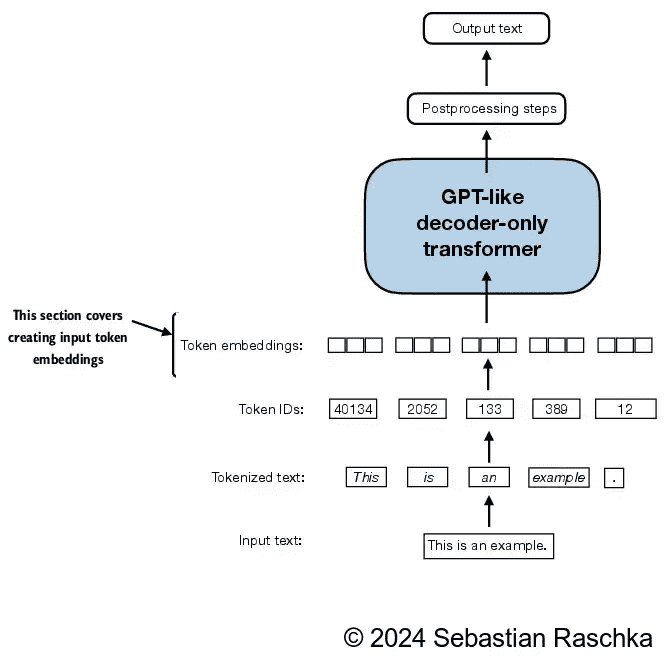
Figure 2.15 Preparing the input text for an LLM involves tokenizing text, converting text tokens to token IDs, and converting token IDs into vector embedding vectors. In this section, we consider the token IDs created in previous sections to create the token embedding vectors.
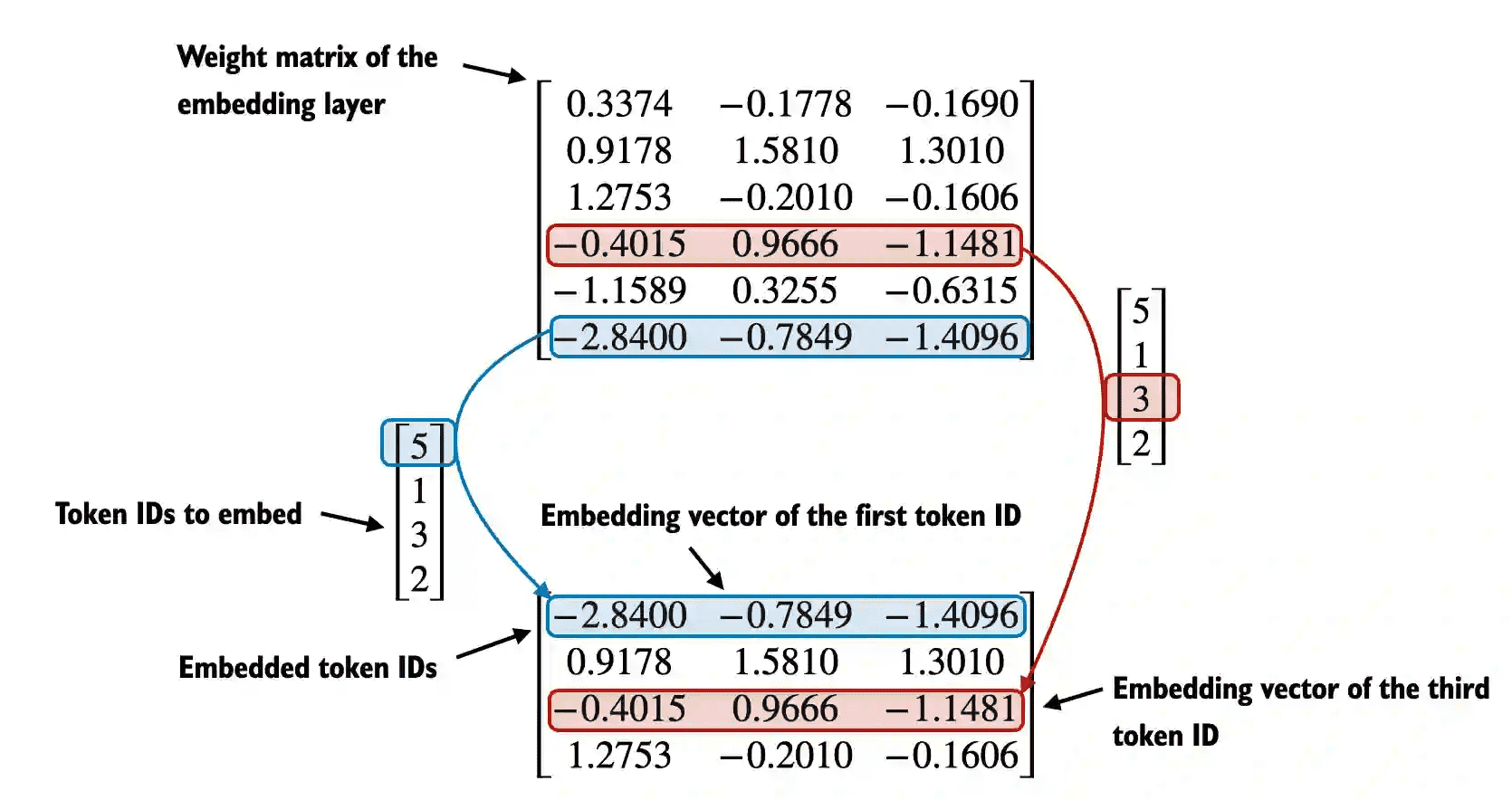
Figure 2.16 Embedding layers perform a look-up operation, retrieving the embedding vector corresponding to the token ID from the embedding layer’s weight matrix. input text => token ID => embedded token ID
2.8 Encoding word positions
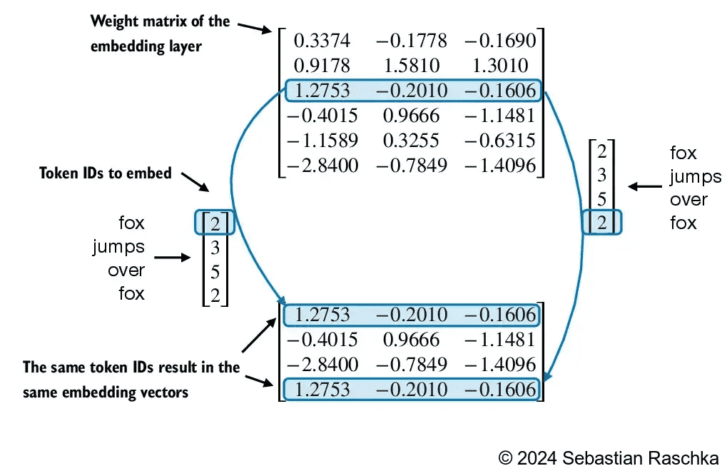
Figure 2.17 The embedding layer converts a token ID into the same vector representation regardless of where it is located in the input sequence. For example, the token ID 2, whether it’s in the first or last position in the token ID input vector, will result in the same embedding vector.
In principle, the deterministic, position-independent embedding of the token ID is good for reproducibility purposes.
However, since the self-attention mechanism of LLMs itself is also position-agnostic, it is helpful to inject additional position information into the LLM.
two broad categories of position-aware embeddings:
1. relative positional embeddings
2. absolute positional embeddings
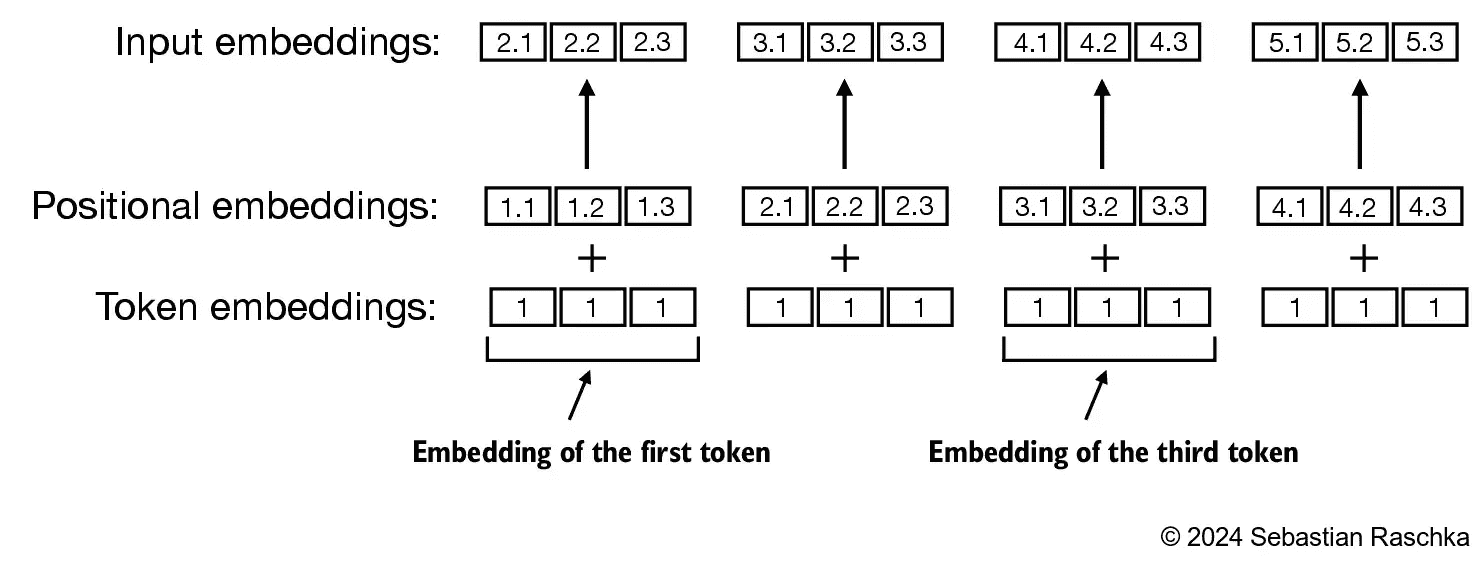
Figure 2.18 Positional embeddings are added to the token embedding vector to create the input embeddings for an LLM. The positional vectors have the same dimension as the original token embeddings. The token embeddings are shown with value 1 for simplicity.
Instead of focusing on the absolute position of a token, the emphasis of relative positional embeddings is on the relative position or distance between tokens. This means the model learns the relationships in terms of “how far apart” rather than “at which exact position.” The advantage here is that the model can generalize better to sequences of varying lengths, even if it hasn’t seen such lengths during training.
OpenAI’s GPT models use absolute positional embeddings that are optimized during the training process rather than being fixed or predefined like the positional encodings in the original Transformer model. This optimization process is part of the model training itself, which we will implement later in this book. For now, let’s create the initial positional embeddings to create the LLM inputs for the upcoming chapters.
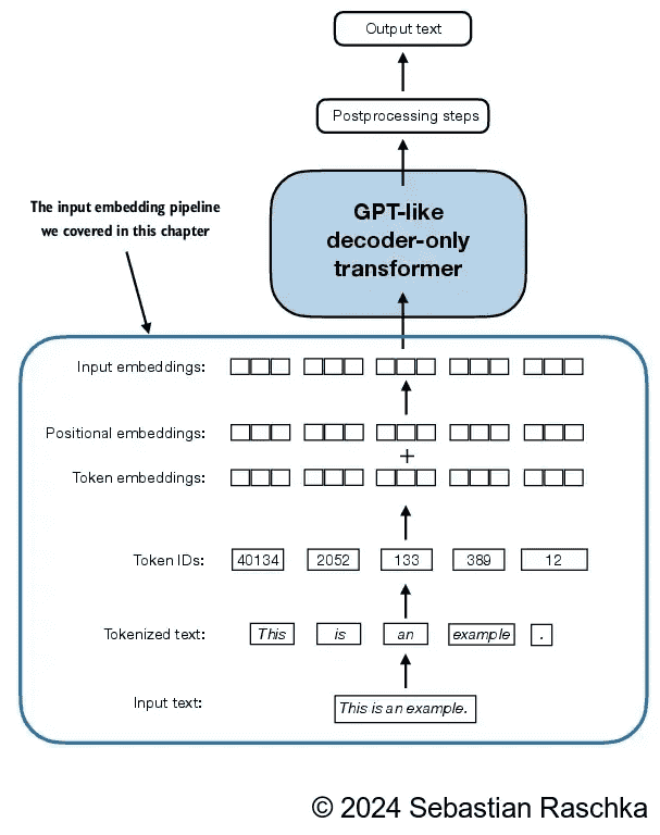
Figure 2.19 As part of the input processing pipeline, input text is first broken up into individual tokens. These tokens are then converted into token IDs using a vocabulary. The token IDs are converted into embedding vectors to which positional embeddings of a similar size are added, resulting in input embeddings that are used as input for the main LLM layers.
context_lengthis a variable that represents the supported input size of the LLM.
2.9 Summary
LLMs require textual data to be converted into numerical vectors, known as embeddings since they can’t process raw text. Embeddings transform discrete data (like words or images) into continuous vector spaces, making them compatible with neural network operations.
As the first step, raw text is broken into tokens, which can be words or characters. Then, the tokens are converted into integer representations, termed token IDs.
Special tokens, such as
<|unk|>and<|endoftext|>, can be added to enhance the model’s understanding and handle various contexts, such as unknown words or marking the boundary between unrelated texts.The
byte pair encoding (BPE)tokenizer used for LLMs like GPT-2 and GPT-3 can efficiently handle unknown words by breaking them down into subword units or individual characters.We use a sliding window approach on tokenized data to generate
input-target pairsfor LLM training.Embedding layers in PyTorch function as a lookup operation, retrieving vectors corresponding to token IDs. The resulting embedding vectors provide continuous representations of tokens, which is crucial for training deep learning models like LLMs.
While token embeddings provide consistent vector representations for each token, they lack a sense of the token’s position in a sequence. To rectify this, two main types of positional embeddings exist: absolute and relative. OpenAI’s GPT models utilize absolute positional embeddings that are added to the token embedding vectors and are optimized during the model training.
3. Coding Attention Mechanisms
Exploring the reasons for using attention mechanisms in neural networks
Introducing a basic self-attention framework and progressing to an enhanced self-attention mechanism
Implementing a causal attention module that allows LLMs to generate one token at a time
Masking randomly selected attention weights with dropout to reduce overfitting
Stacking multiple causal attention modules into a multi-head attention module
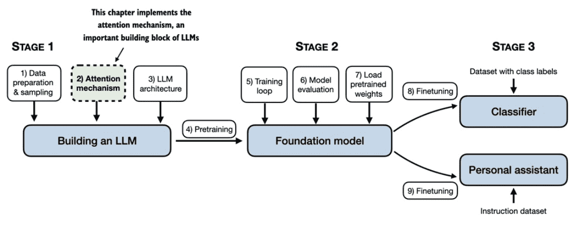
Figure 3.1 A mental model of the three main stages of coding an LLM, pretraining the LLM on a general text dataset, and finetuning it on a labeled dataset. This chapter focuses on attention mechanisms, which are an integral part of an LLM architecture.

Figure 3.2 The figure depicts different attention mechanisms we will code in this chapter, starting with a simplified version of self-attention before adding the trainable weights. The causal attention mechanism adds a mask to self-attention that allows the LLM to generate one word at a time. Finally, multi-head attention organizes the attention mechanism into multiple heads, allowing the model to capture various aspects of the input data in parallel.
3.1 The problem with modeling long sequences
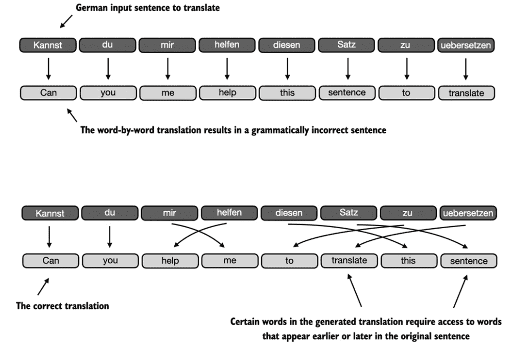
Figure 3.3 When translating text from one language to another, such as German to English, it’s not possible to merely translate word by word. Instead, the translation process requires contextual understanding and grammar alignment.
To address the issue that we cannot translate text word by word, it is common to use a deep neural network with two submodules, a so-called
encoderanddecoder. The job of the encoder is to first read in and process the entire text, and the decoder then produces the translated text. e.g.encoder-decoder RNNs
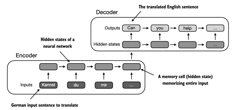
Figure 3.4 Before the advent of transformer models, encoder-decoder RNNs were a popular choice for machine translation. The encoder takes a sequence of tokens from the source language as input, where a hidden state (an intermediate neural network layer) of the encoder encodes a compressed representation of the entire input sequence. Then, the decoder uses its current hidden state to begin the translation, token by token.
The big issue and limitation of encoder-decoder RNNs is that the RNN can’t directly access earlier hidden states from the encoder during the decoding phase. Consequently, it relies solely on the current hidden state, which encapsulates all relevant information. This can lead to a loss of context, especially in complex sentences where dependencies might span long distances.
3.2 Capturing data dependencies with attention mechanisms
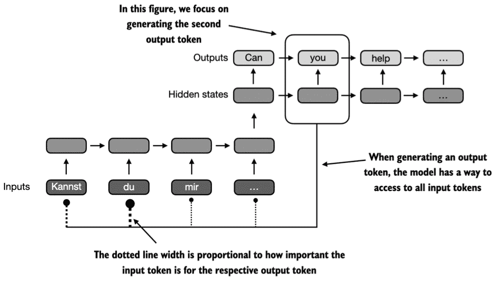
Figure 3.5 Using an attention mechanism, the text-generating decoder part of the network can access all input tokens selectively. This means that some input tokens are more important than others for generating a given output token. The importance is determined by the so-called attention weights, which we will compute later. Note that this figure shows the general idea behind attention and does not depict(描述) the exact implementation of the Bahdanau mechanism, which is an RNN method outside this book’s scope.
Self-attention is a mechanism that allows each position in the input sequence to attend to(注意) all positions in the same sequence when computing the representation of a sequence. Self-attention is a key component of contemporary(当代) LLMs based on the transformer architecture, such as the GPT series.
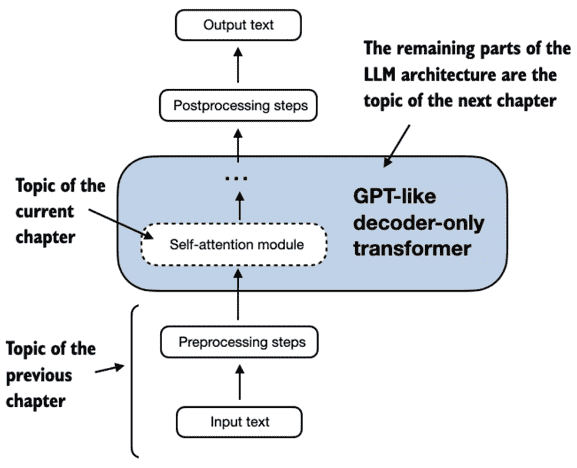
Figure 3.6 Self-attention is a mechanism in transformers that is used to compute more efficient input representations by allowing each position in a sequence to interact with and weigh the importance of all other positions within the same sequence. In this chapter, we will code this self-attention mechanism from the ground up before we code the remaining parts of the GPT-like LLM in the following chapter.
3.3 Attending to different parts of the input with self-attention
The “self” in self-attention
In self-attention, the “self” refers to the mechanism’s ability to compute attention weights by relating different positions within a single input sequence. It assesses and learns the relationships and dependencies between various parts of the input itself, such as words in a sentence or pixels in an image.
This is in contrast to traditional attention mechanisms, where the focus is on the relationships between elements of two different sequences, such as in sequence-to-sequence models where the attention might be between an input sequence and an output sequence, such as the example depicted in Figure 3.5.
3.3.1 A simple self-attention mechanism without trainable weights
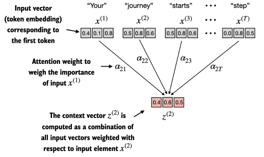
Figure 3.7 The goal of self-attention is to compute a context vector, for each input element, that combines information from all other input elements. In the example depicted in this figure, we compute the context vector \(z^{(2)}\) . The importance or contribution of each input element for computing \(z^{(2)}\) is determined by the attention weights \(α_{21}\) to \(α_{2T}\) . When computing \(z^{(2)}\) , the attention weights are calculated with respect to input element \(x^{(2)}\) and all other inputs. The exact computation of these attention weights is discussed later in this section.
For example, consider an input text like
"Your journey starts with one step."In this case, each element of the sequence, such as \(x^{(1)}\), corresponds to ad-dimensionalembedding vector representing a specific token, like “Your.” These input vectors are shown as3-dimensionalembeddings.Let’s focus on the
embedding vectorof the second input element, \(x^{(2)}\) (which corresponds to the token “journey”), and the correspondingcontext vector, \(z^{(2)}\). This enhancedcontext vector, \(z^{(2)}\), is an embedding that contains information about \(x^{(2)}\) and all other input elements \(x^{(1)}\) to \(x^{(T)}\).In self-attention,
context vectorsplay a crucial role. Their purpose is to create enriched representations of each element in an input sequence (like a sentence) by incorporating information from all other elements in the sequence. This is essential in LLMs, which need to understand the relationship and relevance of words in a sentence to each other. Later, we will add trainable weights that help an LLM learn to construct these context vectors so that they are relevant for the LLM to generate the next token.
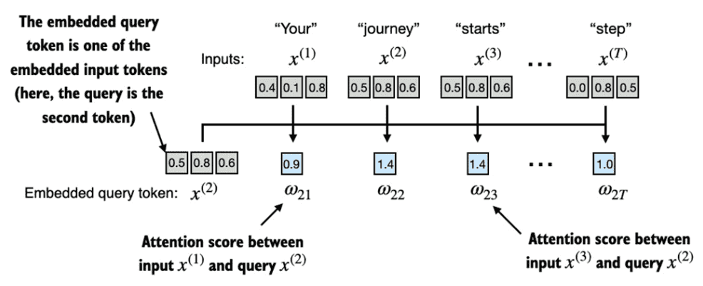
Figure 3.8 The overall goal of this section is to illustrate the computation of the context vector \(z^{(2)}\) using the second input sequence, \(x^{(2)}\) as a query. This figure shows the first intermediate step, computing the attention scores ω between the query \(x^{(2)}\) and all other input elements as a dot product.
import torch
inputs = torch.tensor(
  [[0.43, 0.15, 0.89], # Your     (x^1)
    [0.55, 0.87, 0.66], # journey  (x^2)
    [0.57, 0.85, 0.64], # starts    (x^3)
    [0.22, 0.58, 0.33], # with      (x^4)
    [0.77, 0.25, 0.10], # one       (x^5)
    [0.05, 0.80, 0.55]] # step      (x^6)
)


query = inputs[1]  #A
attn_scores_2 = torch.empty(inputs.shape[0])
for i, x_i in enumerate(inputs):
    attn_scores_2[i] = torch.dot(x_i, query)
print(attn_scores_2)
# 输出
# tensor([0.9544, 1.4950, 1.4754, 0.8434, 0.7070, 1.0865])
除了将点积运算视为组合两个向量以产生标量值的数学工具之外,点积还是相似性的度量,因为它量化了两个向量的对齐程度:更高的点积表示更大程度的对齐或相似性向量之间。在自注意力机制的背景下,点积决定了序列中元素相互关注的程度:点积越高,两个元素之间的相似度和注意力分数就越高。
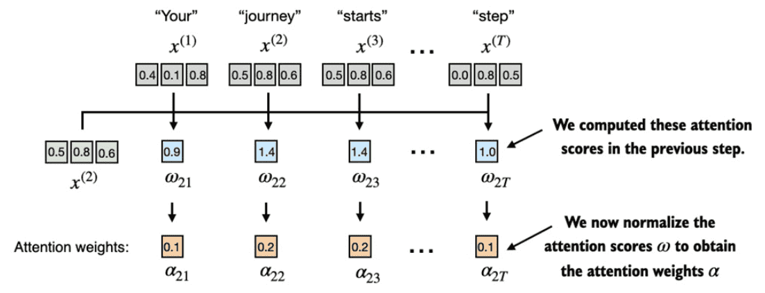
Figure 3.9 After computing the attention scores \(ω_{21}\) to \(ω_{2T}\) with respect to the input query \(x^{(2)}\), the next step is to obtain the attention weights \(α_{21}\) to \(α_{2T}\) by normalizing the attention scores.
标准化背后的主要目标是获得总和为 1 的注意力权重。
attn_weights_2_tmp = attn_scores_2 / attn_scores_2.sum()
print("Attention weights:", attn_weights_2_tmp)
print("Sum:", attn_weights_2_tmp.sum())
# 输出
# Attention weights: tensor([0.1455, 0.2278, 0.2249, 0.1285, 0.1077, 0.1656])
# Sum: tensor(1.0000)
In practice, it’s more common and advisable to use the softmax function for normalization.
In addition, the softmax function ensures that the attention weights are always positive.
def softmax_naive(x):
    return torch.exp(x) / torch.exp(x).sum(dim=0)
attn_weights_2_naive = softmax_naive(attn_scores_2)
print("Attention weights:", attn_weights_2_naive)
print("Sum:", attn_weights_2_naive.sum())
# 输出
# Attention weights: tensor([0.1385, 0.2379, 0.2333, 0.1240, 0.1082, 0.1581])
# Sum: tensor(1.)
Note that this naive softmax implementation (softmax_naive) may encounter numerical instability problems, such as overflow and underflow, when dealing with large or small input values.
PyTorch implementation of softmax
attn_weights_2 = torch.softmax(attn_scores_2, dim=0)
print("Attention weights:", attn_weights_2)
print("Sum:", attn_weights_2.sum())
# 输出
# Attention weights: tensor([0.1385, 0.2379, 0.2333, 0.1240, 0.1082, 0.1581])
# Sum: tensor(1.)
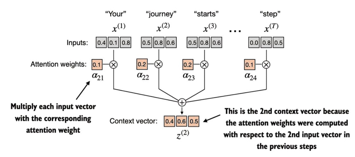
Figure 3.10 The final step, after calculating and normalizing the attention scores to obtain the attention weights for query \(x^{(2)}\), is to compute the context vector \(z^{(2)}\). This context vector is a combination of all input vectors \(x^{(1)}\) to \(x^{(T)}\) weighted by the attention weights.
query = inputs[1] # 2nd input token is the query
context_vec_2 = torch.zeros(query.shape)
for i,x_i in enumerate(inputs):
    context_vec_2 += attn_weights_2[i]*x_i
print(context_vec_2)
# 输出
# tensor([0.4419, 0.6515, 0.5683])
3.3.2 Computing attention weights for all input tokens
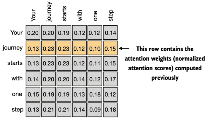
Figure 3.11 The highlighted row shows the attention weights for the second input element as a query, as we computed in the previous section. This section generalizes the computation to obtain all other attention weights.(这是上面用softmax计算出的 attention weights \(α_{21}\) to \(α_{2T}\) )。用同样的方法,可以计算出其他的 attention weights
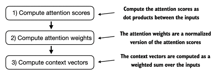
Figure 3.12 计算的3步骤
import torch
inputs = torch.tensor(
  [[0.43, 0.15, 0.89], # Your     (x^1)
    [0.55, 0.87, 0.66], # journey  (x^2)
    [0.57, 0.85, 0.64], # starts    (x^3)
    [0.22, 0.58, 0.33], # with      (x^4)
    [0.77, 0.25, 0.10], # one       (x^5)
    [0.05, 0.80, 0.55]] # step      (x^6)
)

attn_scores = inputs @ inputs.T
print(attn_scores)
# 输出
tensor([[0.9995, 0.9544, 0.9422, 0.4753, 0.4576, 0.6310],
    [0.9544, 1.4950, 1.4754, 0.8434, 0.7070, 1.0865],
    [0.9422, 1.4754, 1.4570, 0.8296, 0.7154, 1.0605],
    [0.4753, 0.8434, 0.8296, 0.4937, 0.3474, 0.6565],
    [0.4576, 0.7070, 0.7154, 0.3474, 0.6654, 0.2935],
    [0.6310, 1.0865, 1.0605, 0.6565, 0.2935, 0.9450]])

attn_weights = torch.softmax(attn_scores, dim=1)
print(attn_weights)
# 输出
tensor([[0.2098, 0.2006, 0.1981, 0.1242, 0.1220, 0.1452],
    [0.1385, 0.2379, 0.2333, 0.1240, 0.1082, 0.1581],
    [0.1390, 0.2369, 0.2326, 0.1242, 0.1108, 0.1565],
    [0.1435, 0.2074, 0.2046, 0.1462, 0.1263, 0.1720],
    [0.1526, 0.1958, 0.1975, 0.1367, 0.1879, 0.1295],
    [0.1385, 0.2184, 0.2128, 0.1420, 0.0988, 0.1896]])

all_context_vecs = attn_weights @ inputs
print(all_context_vecs)
# 输出
tensor([[0.4421, 0.5931, 0.5790],
    [0.4419, 0.6515, 0.5683],
    [0.4431, 0.6496, 0.5671],
    [0.4304, 0.6298, 0.5510],
    [0.4671, 0.5910, 0.5266],
    [0.4177, 0.6503, 0.5645]])
3.4 Implementing self-attention with trainable weights
Self-attention mechanism is also called
scaled dot-product attention.
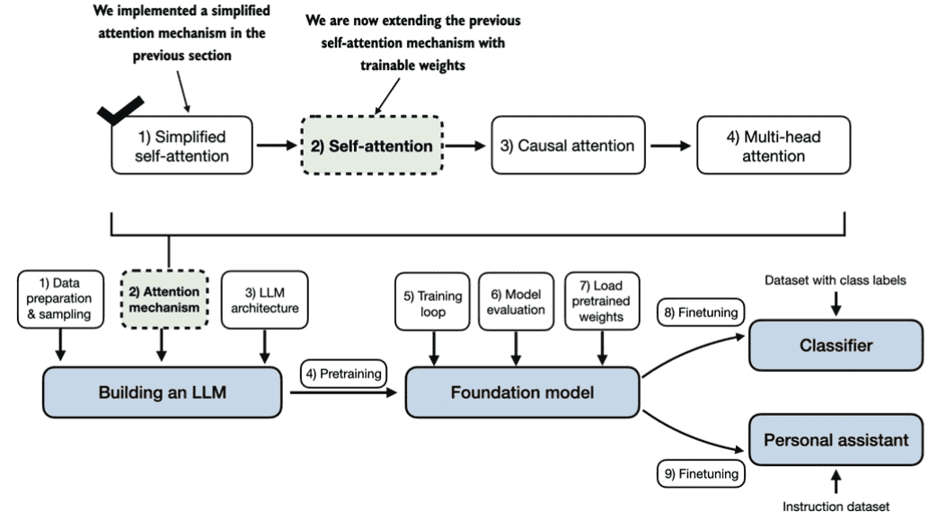
Figure 3.13 A mental model illustrating how the self-attention mechanism we code in this section fits into the broader context of this book and chapter. In the previous section, we coded a simplified attention mechanism to understand the basic mechanism behind attention mechanisms. In this section, we add trainable weights to this attention mechanism. In the upcoming sections, we will then extend this self-attention mechanism by adding a causal mask and multiple heads.
本节主要工作是在前面的基础上增加 训练时更新权重 的功能,以实现在训练时学习以得到更好的权重。
3.4.1 Computing the attention weights step by step
three trainable weight matrices \(W_q\) , \(W_k\) , and \(W_v\) .
These three matrices are used to project the embedded input tokens, \(x^{(i)}\), into query, key, and value vectors

Figure 3.14 In the first step of the self-attention mechanism with trainable weight matrices, we compute query (q), key (k), and value (v) vectors for input elements x. Similar to previous sections, we designate the second input, \(x^{(2)}\), as the query input. The query vector \(q^{(2)}\) is obtained via matrix multiplication between the input \(x^{(2)}\) and the weight matrix Wq. Similarly, we obtain the key and value vectors(即: \(k^{(T)}\) and \(v^{(T)}\) ) via matrix multiplication involving the weight matrices Wk and Wv.
Note that in GPT-like models, the input and output dimensions are usually the same, but for illustration purposes, to better follow the computation, we choose different input (d_in=3) and output (d_out=2) dimensions here.
import torch
inputs = torch.tensor(
  [[0.43, 0.15, 0.89], # Your     (x^1)
    [0.55, 0.87, 0.66], # journey  (x^2)
    [0.57, 0.85, 0.64], # starts    (x^3)
    [0.22, 0.58, 0.33], # with      (x^4)
    [0.77, 0.25, 0.10], # one       (x^5)
    [0.05, 0.80, 0.55]] # step      (x^6)
)

x_2 = inputs[1] #A
d_in = inputs.shape[1] #B  = 3
d_out = 2 #C

# Initialize the three weight matrices Wq, Wk, and Wv
torch.manual_seed(123)
W_query = torch.nn.Parameter(torch.rand(d_in, d_out), requires_grad=False)
W_key   = torch.nn.Parameter(torch.rand(d_in, d_out), requires_grad=False)
W_value = torch.nn.Parameter(torch.rand(d_in, d_out), requires_grad=False)
# 示例结构: shape=(3,2)
# tensor([[0.3821, 0.6605],
#         [0.8536, 0.5932],
#         [0.6367, 0.9826]])
# 说明
# setting requires_grad=False to reduce clutter in the outputs for illustration purposes
# 正式使用时需要设置 requires_grad=True

# compute the query, key, and value vectors
query_2 = x_2 @ W_query
key_2 = x_2 @ W_key
value_2 = x_2 @ W_value
print(query_2)
# 输出
# tensor([0.4306, 1.4551])
【注意】不要将权重参数(weight parameters)与注意力权重(attention weights)混淆。
权重参数(weight parameters): 指的是神经网络在训练过程中被调优的权重,有时会缩写为weight。(“weight” is short for “weight parameters,” the values of a neural network that are optimized during training. )
注意力权重(attention weights): 决定了上下文向量依赖输入不同部分的程度,即网络关注输入不同部分的程度。(attention weights determine the extent to which a context vector depends on the different parts of the input, i.e., to what extent the network focuses on different parts of the input.)
总之,权重参数是定义网络连接的基本学习系数,而注意力权重是动态的、特定于上下文的值。
# 虽然这儿只计算context vector`Z^(2)`,但仍然需要所有输入元素的键和值向量
# obtain all keys and values via matrix multiplication
keys = inputs @ W_key
values = inputs @ W_value
print("keys.shape:", keys.shape)
# 输出
# keys.shape: torch.Size([6, 2])
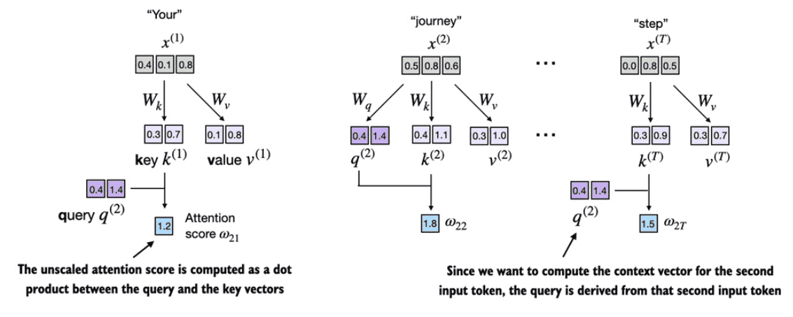
Figure 3.15 The attention score computation is a dot-product computation similar to what we have used in the simplified self-attention mechanism in section 3.3. The new aspect here is that we are not directly computing the dot-product between the input elements but using the query and key obtained by transforming the inputs via the respective weight matrices.
compute the
attention score\(ω_{22}\)
keys_2 = keys[1] #A
attn_score_22 = query_2.dot(keys_2)
print(attn_score_22)
# tensor(1.8524)
同样的道理计算出所有的 \(ω_2\) (即 \(ω_{21}\) 到 \(ω_{2T}\) )
attn_scores_2 = query_2 @ keys.T    # All attention scores for given query
print(attn_scores_2)
# 输出
# tensor([1.2705, 1.8524, 1.8111, 1.0795, 0.5577, 1.5440])
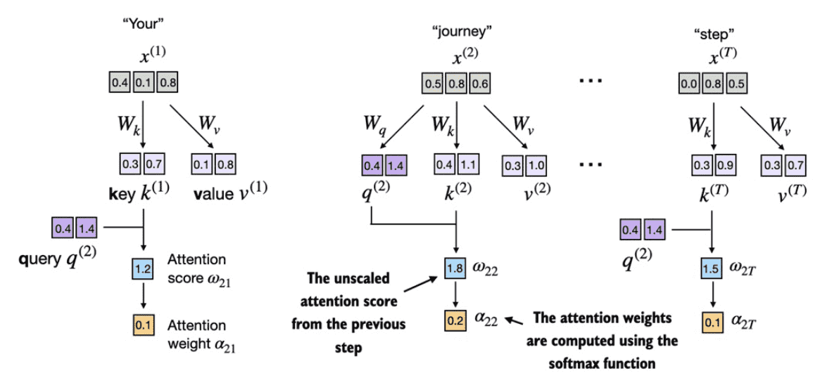
Figure 3.16 After computing the attention scores ω, the next step is to normalize these scores using the softmax function to obtain the attention weights α.
d_k = keys.shape[-1]
attn_weights_2 = torch.softmax(attn_scores_2 / d_k**0.5, dim=-1)
print(attn_weights_2)
# 输出
# tensor([0.1500, 0.2264, 0.2199, 0.1311, 0.0906, 0.1820])
通过将注意力分数除以嵌入的平方根(square root, 即d_k**0.5)来缩放注意力分数键的维度
when scaling up the embedding dimension, which is typically greater than thousand(比较gpt4等), large dot products can result in very small gradients during backpropagation due to the softmax function applied to them.
As dot products increase, the softmax function behaves more like a step function, resulting in gradients nearing zero.
These small gradients can drastically slow down learning or cause training to stagnate.
The scaling by the
square rootof the embedding dimension is the reason why this self-attention mechanism is also calledscaled-dot product attention.【关键点】为什么在自注意力机制中会用嵌入维度的平方根来缩放点积
缩放的目的:用嵌入维度的平方根来缩放,是为了避免训练过程中出现过小的梯度。若不做缩放,训练时可能会遇到梯度非常小的情况,导致模型学习变慢,甚至陷入停滞。
出现梯度变小的原因:1、当嵌入维度(即向量的维度)增加时,两个向量的点积值会变大。在GPT等大型语言模型(LLM)中,嵌入维度往往很高,可能达到上千,因此点积也变得很大。2、在点积结果上应用 softmax 函数时,如果数值较大,softmax 输出的概率分布会变得很尖锐,近似于阶跃函数。此时,大部分概率集中在几个值上,导致其他部分的梯度几乎为零。这样就会导致模型训练时更新不充分。
缩放的效果:通过用嵌入维度的平方根缩放点积的大小,可以让点积的数值控制在合理范围,使得 softmax 函数的输出更加平滑,从而使得梯度较大,模型可以更有效地学习。这种缩放的自注意力机制因此被称为“缩放点积注意力” (scaled-dot product attention)。
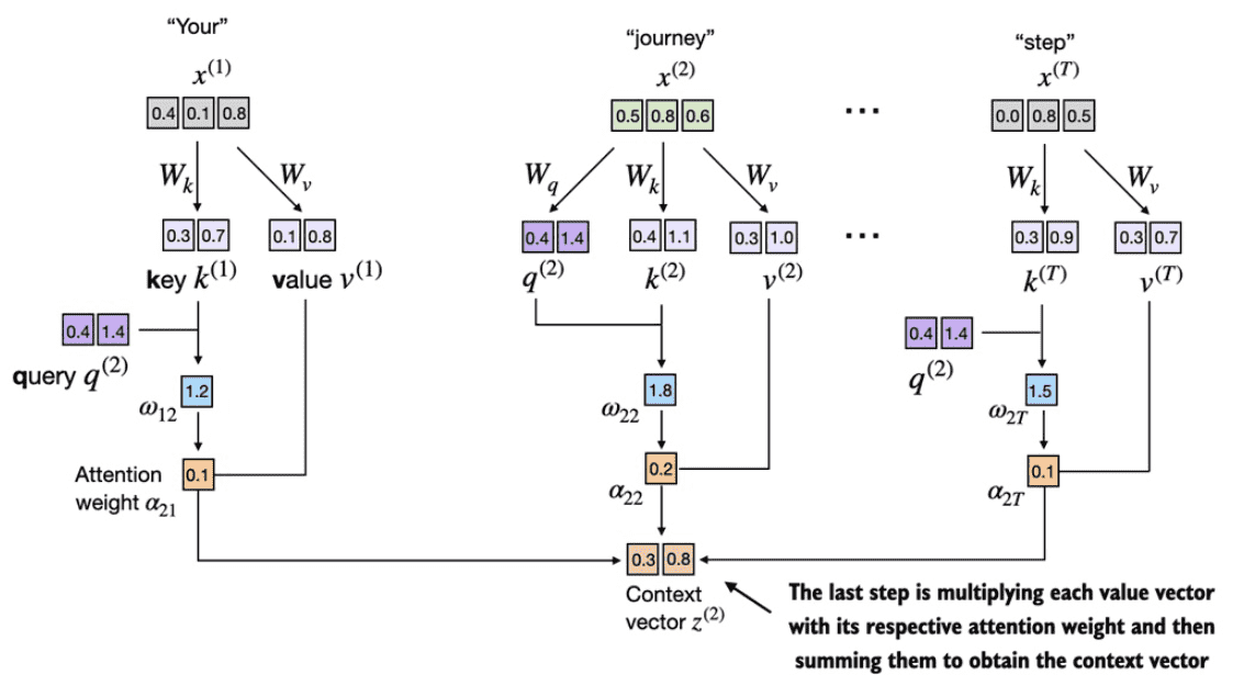
Figure 3.17 In the final step of the self-attention computation, we compute the context vector by combining all value vectors via the attention weights.
context_vec_2 = attn_weights_2 @ values
print(context_vec_2)
# 输出
# tensor([0.3061, 0.8210])
备注
【为啥需要query, key, and value】这3个是借用信息检索和数据库领域的概念。接合起来理解这3个概念。
query(查询):”query” 代表模型当前关注的项(如一个句子中的单词或词元)。模型通过 “query” 来探测其他部分,判断需要关注的程度。
key(键):输入序列中的每个项(如句子中的每个词)都有一个对应的 “key”,这些 “key” 会和 “query” 进行匹配。通过这种匹配,模型可以找出哪些 “key”(即哪些输入部分)和 “query” 更相关。
value(值):一旦模型确定了与 “query” 最相关的 “key”,就会取出相应的 “value”。这些 “value” 包含输入项的实际内容或表示,通过提取这些 “value”,模型获得当前 “query” 应关注的具体内容。
备注
上节讲的是根据 关系相近的向量点积更大 与计算相似度的关系,算出每个单词的权重,然后用这个计算出的权重和输入向量点击,得到与位置相关的上下文向量。而本节是用3个可训练参数(Wq, Wk, Wv),由Wq和Wk来计算出每个单词的权重,而Wv提供了该位置上的特征信息,模型通过注意力机制自动调整从不同位置的 value 中提取多少信息。
注:为啥 Wv 不能直接用 input来表示,因为 Wv 直接决定了提取的内容和最终输出的特征信息。它能够捕捉更复杂的特征,尤其是在上下文依赖和长序列建模中,可以更好地识别出不同位置特征的细微差别。直接使用 input,模型会缺乏这种内容和注意力分布的区分,使得不同位置的特征难以有效加权合成,从而降低注意力机制的表达能力。
3.4.2 Implementing a compact self-attention Python class
Listing 3.1 A compact self-attention class
import torch.nn as nn
class SelfAttention_v1(nn.Module):
    def __init__(self, d_in, d_out):
        super().__init__()
        self.d_out = d_out
        self.W_query = nn.Parameter(torch.rand(d_in, d_out))
        self.W_key   = nn.Parameter(torch.rand(d_in, d_out))
        self.W_value = nn.Parameter(torch.rand(d_in, d_out))
    def forward(self, x):
        keys = x @ self.W_key
        queries = x @ self.W_query
        values = x @ self.W_value

        attn_scores = queries @ keys.T # omega

        attn_weights = torch.softmax(
            attn_scores / keys.shape[-1]**0.5, dim=-1)

        context_vec = attn_weights @ values
        return context_vec

torch.manual_seed(123)
sa_v1 = SelfAttention_v1(d_in, d_out)
print(sa_v1(inputs))
# 输出
tensor([[0.2996, 0.8053],
        [0.3061, 0.8210],
        [0.3058, 0.8203],
        [0.2948, 0.7939],
        [0.2927, 0.7891],
        [0.2990, 0.8040]], grad_fn=<MmBackward0>)
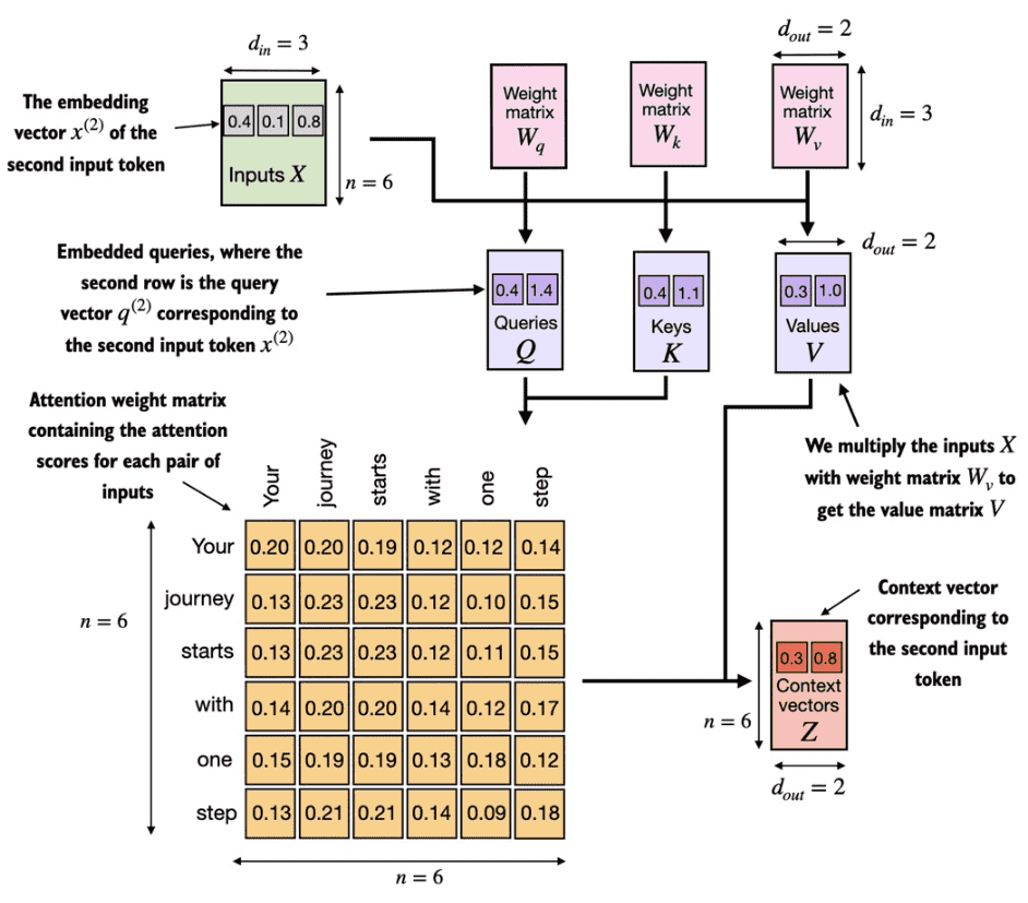
Figure 3.18 In self-attention, we transform the input vectors in the input matrix X with the three weight matrices, Wq, Wk, and Wv. Then, we compute the attention weight matrix based on the resulting queries (Q) and keys (K). Using the attention weights and values (V), we then compute the context vectors (Z). (For visual clarity, we focus on a single input text with n tokens in this figure, not a batch of multiple inputs. Consequently, the 3D input tensor is simplified to a 2D matrix in this context. This approach allows for a more straightforward visualization and understanding of the processes involved.)
Using
nn.Linearinstead of manually implementingnn.Parameter(torch.rand(...))is thatnn.Linearhas an optimized weight initialization scheme, contributing to more stable and effective model training.Listing 3.2 A self-attention class using PyTorch’s Linear layers
class SelfAttention_v2(nn.Module):
    def __init__(self, d_in, d_out, qkv_bias=False):
        super().__init__()
        self.d_out = d_out
        self.W_query = nn.Linear(d_in, d_out, bias=qkv_bias)
        self.W_key   = nn.Linear(d_in, d_out, bias=qkv_bias)
        self.W_value = nn.Linear(d_in, d_out, bias=qkv_bias)
    def forward(self, x):
        keys = self.W_key(x)
        queries = self.W_query(x)
        values = self.W_value(x)

        attn_scores = queries @ keys.T

        attn_weights = torch.softmax(attn_scores / keys.shape[-1]**0.5, dim)

        context_vec = attn_weights @ values
        return context_vec

torch.manual_seed(789)
sa_v2 = SelfAttention_v2(d_in, d_out)
print(sa_v2(inputs))
# 输出
tensor([[-0.0739,  0.0713],
        [-0.0748,  0.0703],
        [-0.0749,  0.0702],
        [-0.0760,  0.0685],
        [-0.0763,  0.0679],
        [-0.0754,  0.0693]], grad_fn=<MmBackward0>)
Note that SelfAttention_v1 and SelfAttention_v2 give different outputs because they use different initial weights for the weight matrices since nn.Linear uses a more sophisticated weight initialization scheme.
3.5 Hiding future words with causal attention
Causal attention, also known asmasked attention, is a specialized form of self-attention. It restricts a model to only consider previous and current inputs in a sequence when processing any given token. This is in contrast to the standard self-attention mechanism, which allows access to the entire input sequence at once.
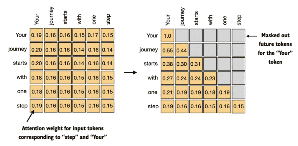
Figure 3.19 In causal attention, we mask out the attention weights above the diagonal such that for a given input, the LLM can’t access future tokens when computing the context vectors using the attention weights. For example, for the word “journey” in the second row, we only keep the attention weights for the words before (“Your”) and in the current position (“journey”).
3.5.1 Applying a causal attention mask

Figure 3.20 One way to obtain the masked attention weight matrix in causal attention is to apply the softmax function to the attention scores, zeroing out the elements above the diagonal and normalizing the resulting matrix.
【第一步】使用上面的方法得到 attention weights
print(attn_weights)
tensor([[0.1921, 0.1646, 0.1652, 0.1550, 0.1721, 0.1510],
        [0.2041, 0.1659, 0.1662, 0.1496, 0.1665, 0.1477],
        [0.2036, 0.1659, 0.1662, 0.1498, 0.1664, 0.1480],
        [0.1869, 0.1667, 0.1668, 0.1571, 0.1661, 0.1564],
        [0.1830, 0.1669, 0.1670, 0.1588, 0.1658, 0.1585],
        [0.1935, 0.1663, 0.1666, 0.1542, 0.1666, 0.1529]],
grad_fn=<SoftmaxBackward0>)
【第二步】对象线上面的设置为0
context_length = attn_scores.shape[0]
mask_simple = torch.tril(torch.ones(context_length, context_length))
print(mask_simple)
# 输出
tensor([[1., 0., 0., 0., 0., 0.],
        [1., 1., 0., 0., 0., 0.],
        [1., 1., 1., 0., 0., 0.],
        [1., 1., 1., 1., 0., 0.],
        [1., 1., 1., 1., 1., 0.],
        [1., 1., 1., 1., 1., 1.]])

# multiply this mask with the attention weights
masked_simple = attn_weights*mask_simple
print(masked_simple)
# 输出
tensor([[0.1921, 0.0000, 0.0000, 0.0000, 0.0000, 0.0000],
        [0.2041, 0.1659, 0.0000, 0.0000, 0.0000, 0.0000],
        [0.2036, 0.1659, 0.1662, 0.0000, 0.0000, 0.0000],
        [0.1869, 0.1667, 0.1668, 0.1571, 0.0000, 0.0000],
        [0.1830, 0.1669, 0.1670, 0.1588, 0.1658, 0.0000],
        [0.1935, 0.1663, 0.1666, 0.1542, 0.1666, 0.1529]],
       grad_fn=<MulBackward0>)
【第三步】重新规范化(renormalize) attention weights使每一行值的和为1
row_sums = masked_simple.sum(dim=1, keepdim=True)
masked_simple_norm = masked_simple / row_sums
print(masked_simple_norm)
# 输出
tensor([[1.0000, 0.0000, 0.0000, 0.0000, 0.0000, 0.0000],
        [0.5517, 0.4483, 0.0000, 0.0000, 0.0000, 0.0000],
        [0.3800, 0.3097, 0.3103, 0.0000, 0.0000, 0.0000],
        [0.2758, 0.2460, 0.2462, 0.2319, 0.0000, 0.0000],
        [0.2175, 0.1983, 0.1984, 0.1888, 0.1971, 0.0000],
        [0.1935, 0.1663, 0.1666, 0.1542, 0.1666, 0.1529]],
       grad_fn=<DivBackward0>)
【注意-信息泄露】当我们应用掩码然后重新规范化注意力权重时,最初来自未来标记(现在已经掩码)的信息仍然可能影响当前标记,因为它们的值是 softmax 计算的一部分。然而,关键的洞察是,当我们在屏蔽后重新规范化注意力权重时,我们本质上所做的是在较小的子集上重新计算 softmax(因为屏蔽位置对 softmax 值没有贡献)。Softmax 的数学优雅之处在于,尽管最初在分母中包含了所有位置,但在屏蔽和重新归一化之后,屏蔽位置的影响被抵消了——它们不会以任何有意义的方式对 SoftMax 得分做出贡献。所以不会有信息泄露。

Figure 3.21 A more efficient way to obtain the masked attention weight matrix in causal attention is to mask the attention scores with negative infinity values before applying the softmax function.
这儿可以利用 softmax 函数的数学特性,以更少的步骤更有效地实现屏蔽注意力权重的计算
【关键特征】当负无穷大值 (-∞) 连续存在时,softmax 函数将它们视为零概率(从数学上讲,这是因为 \(e^{-\infty}\) 接近 0)。
这儿把上面的0改为
-∞(即-inf)
mask = torch.triu(torch.ones(context_length, context_length), diagonal=1)
masked = attn_scores.masked_fill(mask.bool(), -torch.inf)
print(masked)
# 输出
tensor([[0.2899,   -inf,   -inf,   -inf,   -inf,   -inf],
        [0.4656, 0.1723,   -inf,   -inf,   -inf,   -inf],
        [0.4594, 0.1703, 0.1731,   -inf,   -inf,
        [0.2642, 0.1024, 0.1036, 0.0186,   -inf,
        [0.2183, 0.0874, 0.0882, 0.0177, 0.0786,
        [0.3408, 0.1270, 0.1290, 0.0198, 0.1290, 0.0078]],
       grad_fn=<MaskedFillBackward0>)


attn_weights = torch.softmax(masked / keys.shape[-1]**0.5, dim=1)
print(attn_weights)
# 输出(已经规范化,不用再额外操作了,节省了操作)
tensor([[1.0000, 0.0000, 0.0000, 0.0000, 0.0000, 0.0000],
        [0.5517, 0.4483, 0.0000, 0.0000, 0.0000, 0.0000],
        [0.3800, 0.3097, 0.3103, 0.0000, 0.0000, 0.0000],
        [0.2758, 0.2460, 0.2462, 0.2319, 0.0000, 0.0000],
        [0.2175, 0.1983, 0.1984, 0.1888, 0.1971, 0.0000],
        [0.1935, 0.1663, 0.1666, 0.1542, 0.1666, 0.1529]],
       grad_fn=<SoftmaxBackward0>)
3.5.2 Masking additional attention weights with dropout
Dropout in deep learning is a technique where randomly selected hidden layer units are ignored during training, effectively “dropping” them out. This method helps prevent overfitting by ensuring that a model does not become overly reliant on any specific set of hidden layer units. It’s important to emphasize that dropout is only used during training and is disabled afterward.
备注
In the transformer architecture, including models like GPT, dropout in the attention mechanism is typically applied in two specific areas: after calculating the attention scores or after applying the attention weights to the value vectors.(我还没完全理解具体的位置)
我的理解(GPT给的说法有矛盾,下面是我的理解)
【Dropout 的应用位置】1、after calculating the attention scores:在计算注意力分数后应用Dropout意味着在得到Q(查询)、K(键)和V(值)向量之间的点积之后,但在将这些分数传递给Softmax函数之前,进行Dropout操作。这一步骤中的Dropout可以帮助模型避免对某些特定特征的过度依赖,因为它可能会随机地使一些注意力分数失效,从而促使模型学习到更加健壮的注意力分布。
伪代码:
function scaledDotProductAttention(Q, K, V, dropoutRate):
    # 计算注意力分数
    scores = matmul(Q, transpose(K)) / sqrt(d_k)  # d_k 是键向量的维度

    # 应用Dropout
    scores = applyDropout(scores, dropoutRate)

    # 应用Softmax函数
    attentionWeights = softmax(scores)

    # 将注意力权重应用到值向量上
    output = matmul(attentionWeights, V)

    return output
【Dropout 的应用位置】2、after applying the attention weights to the value vectors:在将注意力权重应用到值向量之后应用Dropout意味着在Softmax后的注意力权重与值向量相乘得到加权值向量之后,再执行Dropout操作。这样做可以进一步帮助模型泛化,因为即使某些信息被Dropout随机丢弃了,模型仍然需要能够利用剩余的信息来做出准确的预测。
伪代码:
function scaledDotProductAttention(Q, K, V, dropoutRate):
    # 计算注意力分数
    scores = matmul(Q, transpose(K)) / sqrt(d_k)  # d_k 是键向量的维度

    # 应用Softmax函数
    attentionWeights = softmax(scores)

    # 应用Dropout
    attentionWeights = applyDropout(attentionWeights, dropoutRate)

    # 将注意力权重应用到值向量上
    output = matmul(attentionWeights, V)

    return output
备注
下面示例演示了 “apply the dropout mask after computing the attention weights”
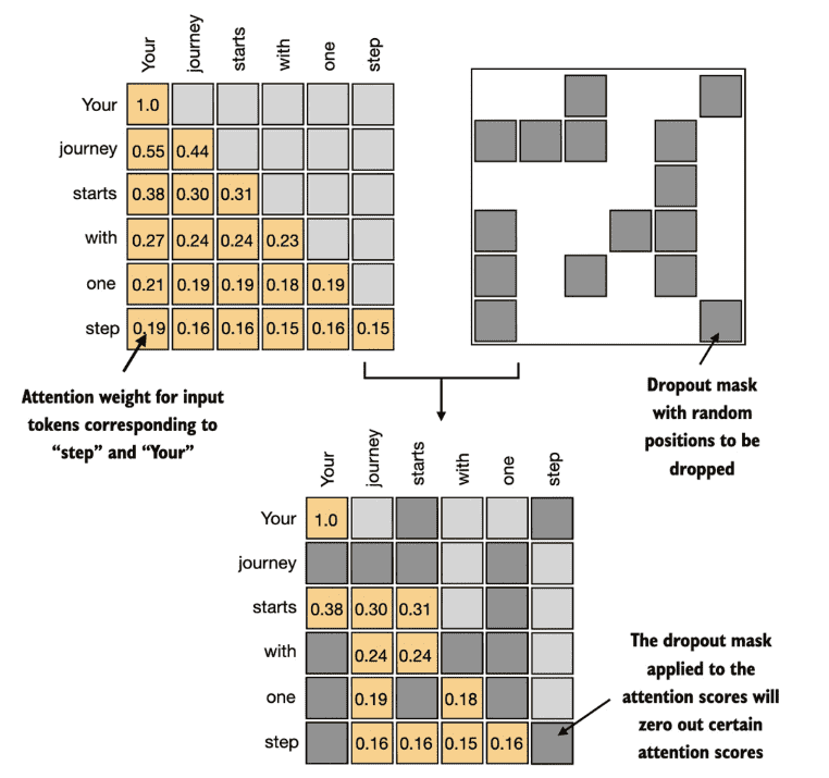
Figure 3.22 Using the causal attention mask (upper left), we apply an additional dropout mask (upper right) to zero out additional attention weights to reduce overfitting during training.
在下面的示例中我们dropout 50% 的比例,在后面训练gpt 模型时,我们使用 10%-20% 的 dropout 比例。
torch.manual_seed(123)
dropout = torch.nn.Dropout(0.5) #A
example = torch.ones(6, 6) #B
print(dropout(example))
# 输出(有近一半是0)
tensor([[2., 2., 0., 2., 2., 0.],
        [0., 0., 0., 2., 0., 2.],
        [2., 2., 2., 2., 0., 2.],
        [0., 2., 2., 0., 0., 2.],
        [0., 2., 0., 2., 0., 2.],
        [0., 2., 2., 2., 2., 0.]])
apply dropout to the attention weight matrix:
torch.manual_seed(123)
print(dropout(attn_weights))
# 输出
tensor([[2.0000, 0.0000, 0.0000, 0.0000, 0.0000, 0.0000],
        [0.0000, 0.0000, 0.0000, 0.0000, 0.0000, 0.0000],
        [0.7599, 0.6194, 0.6206, 0.0000, 0.0000, 0.0000],
        [0.0000, 0.4921, 0.4925, 0.0000, 0.0000, 0.0000],
        [0.0000, 0.3966, 0.0000, 0.3775, 0.0000, 0.0000],
        [0.0000, 0.3327, 0.3331, 0.3084, 0.3331, 0.0000]],
       grad_fn=<MulBackward0>
3.5.3 Implementing a compact causal attention class
Listing 3.3 A compact causal attention class
class CausalAttention(nn.Module):

    def __init__(self, d_in, d_out, context_length,
                 dropout, qkv_bias=False):
        super().__init__()
        self.d_out = d_out
        self.W_query = nn.Linear(d_in, d_out, bias=qkv_bias)
        self.W_key   = nn.Linear(d_in, d_out, bias=qkv_bias)
        self.W_value = nn.Linear(d_in, d_out, bias=qkv_bias)
        self.dropout = nn.Dropout(dropout) # A
        self.register_buffer(
            'mask',
            torch.triu(
                torch.ones(context_length, context_length),
                diagonal=1
            )
        ) #B


    def forward(self, x):
        b, num_tokens, d_in = x.shape  #C
        keys = self.W_key(x)
        queries = self.W_query(x)
        values = self.W_value(x)

        attn_scores = queries @ keys.transpose(1, 2)  #C
        attn_scores.masked_fill_(  #D
            self.mask.bool()[:num_tokens, :num_tokens], -torch.inf)
        attn_weights = torch.softmax(attn_scores / keys.shape[-1]**0.5, dim=-1)
        attn_weights = self.dropout(attn_weights)

        context_vec = attn_weights @ values
        return context_vec


import torch
inputs = torch.tensor(
  [[0.43, 0.15, 0.89], # Your     (x^1)
   [0.55, 0.87, 0.66], # journey  (x^2)
   [0.57, 0.85, 0.64], # starts   (x^3)
   [0.22, 0.58, 0.33], # with     (x^4)
   [0.77, 0.25, 0.10], # one      (x^5)
   [0.05, 0.80, 0.55]] # step     (x^6)
)
batch = torch.stack((inputs, inputs), dim=0)

torch.manual_seed(123)
context_length = batch.shape[1]
ca = CausalAttention(d_in, d_out, context_length, 0.0)
context_vecs = ca(batch)
print("context_vecs.shape:", context_vecs.shape)
# 输出
# context_vecs.shape: torch.Size([2, 6, 2])

Figure 3.23 A mental model summarizing the four different attention modules we are coding in this chapter. We began with a simplified attention mechanism, added trainable weights, and then added a casual attention mask. In the remainder of this chapter, we will extend the causal attention mechanism and code multi-head attention, which is the final module we will use in the LLM implementation in the next chapter.
3.6 Extending single-head attention to multi-head attention
3.6.1 Stacking multiple single-head attention layers
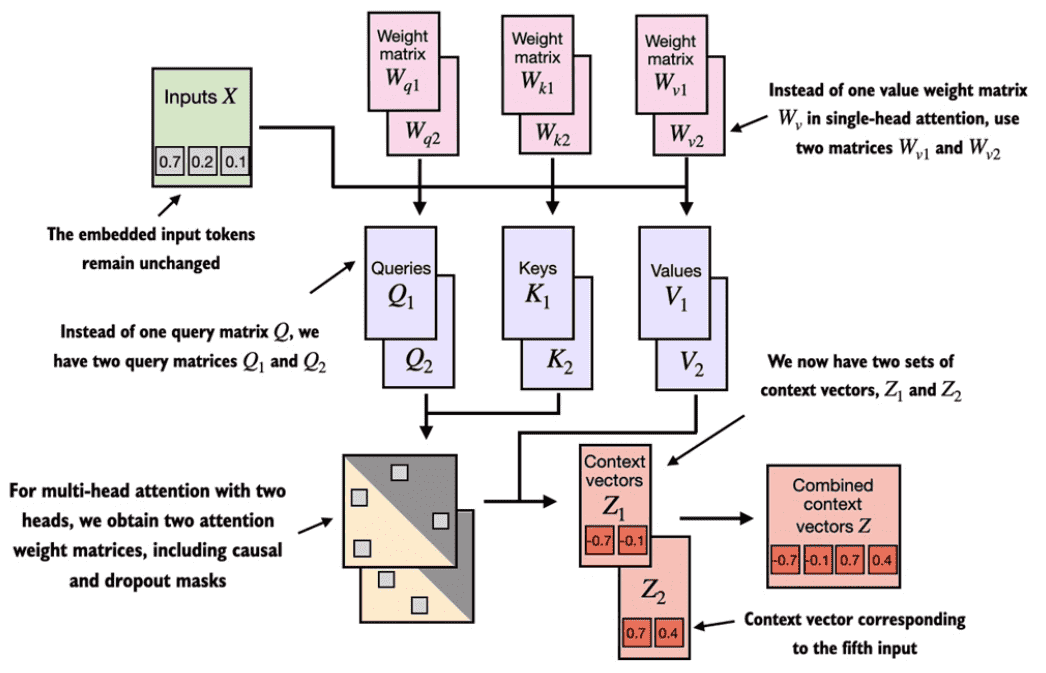
Figure 3.24 The multi-head attention module in this figure depicts two single-head attention modules stacked on top of each other. So, instead of using a single matrix Wv for computing the value matrices, in a multi-head attention module with two heads, we now have two value weight matrices: \(W_{v1}\) and \(W_{v2}\). The same applies to the other weight matrices, Wq and Wk. We obtain two sets of context vectors Z1 and Z2 that we can combine into a single context vector matrix Z.
Listing 3.4 A wrapper class to implement multi-head attention
class MultiHeadAttentionWrapper(nn.Module):
    def __init__(self, d_in, d_out, context_length, dropout, num_heads, qkv_bias=False):
        super().__init__()
        self.heads = nn.ModuleList(
            [CausalAttention(d_in, d_out, context_length, dropout, qkv_bias)
             for _ in range(num_heads)]
        )

    def forward(self, x):
        return torch.cat([head(x) for head in self.heads], dim=-1)
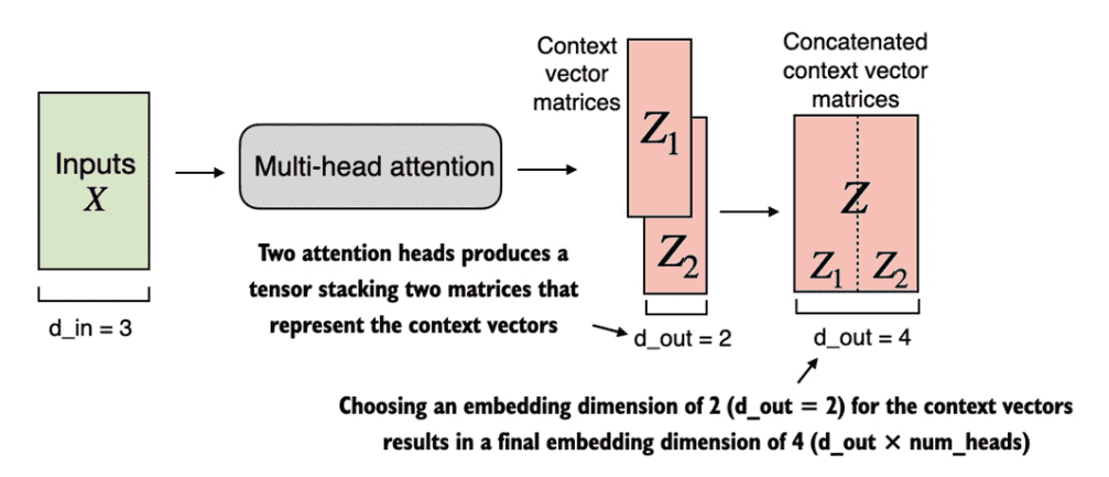
Figure 3.25 Using the MultiHeadAttentionWrapper, we specified the number of attention heads (num_heads). If we set num_heads=2, as shown in this figure, we obtain a tensor with two sets of context vector matrices. In each context vector matrix, the rows represent the context vectors corresponding to the tokens, and the columns correspond to the embedding dimension specified via d_out=4. We concatenate these context vector matrices along the column dimension. Since we have 2 attention heads and an embedding dimension of 2, the final embedding dimension is 2 × 2 = 4.
torch.manual_seed(123)

context_length = batch.shape[1] # This is the number of tokens
d_in, d_out = 3, 2
mha = MultiHeadAttentionWrapper(
    d_in, d_out, context_length, 0.0, num_heads=2
)

context_vecs = mha(batch)

print("context_vecs.shape:", context_vecs.shape)
#context_vecs.shape: torch.Size([2, 6, 4])
print(context_vecs)
# 输出
# tensor([[[-0.4519,  0.2216,  0.4772,  0.1063],
#          [-0.5874,  0.0058,  0.5891,  0.3257],
#          [-0.6300, -0.0632,  0.6202,  0.3860],
#          [-0.5675, -0.0843,  0.5478,  0.3589],
#          [-0.5526, -0.0981,  0.5321,  0.3428],
#          [-0.5299, -0.1081,  0.5077,  0.3493]],

#         [[-0.4519,  0.2216,  0.4772,  0.1063],
#          [-0.5874,  0.0058,  0.5891,  0.3257],
#          [-0.6300, -0.0632,  0.6202,  0.3860],
#          [-0.5675, -0.0843,  0.5478,  0.3589],
#          [-0.5526, -0.0981,  0.5321,  0.3428],
#          [-0.5299, -0.1081,  0.5077,  0.3493]]], grad_fn=<CatBackward0>)

# 说明
# first  dimension: context_vecs tensor is 2 since we have two input texts
#       (两个值完全一样是因为输入文本batch, 是完全一样的)
# second dimension: 6 tokens in each input
# third  dimension: 4-dimensional embedding of each token
3.6.2 Implementing multi-head attention with weight splits
class MultiHeadAttention(nn.Module):
    def __init__(self, d_in, d_out, context_length, dropout, num_heads, qkv_bias=False):
        super().__init__()
        assert (d_out % num_heads == 0), \
            "d_out must be divisible by num_heads"

        self.d_out = d_out
        self.num_heads = num_heads
        self.head_dim = d_out // num_heads  # Reduce the projection dim to match desired output dim

        self.W_query = nn.Linear(d_in, d_out, bias=qkv_bias)
        self.W_key = nn.Linear(d_in, d_out, bias=qkv_bias)
        self.W_value = nn.Linear(d_in, d_out, bias=qkv_bias)
        self.out_proj = nn.Linear(d_out, d_out)  # Linear layer to combine head outputs
        self.dropout = nn.Dropout(dropout)
        self.register_buffer(
            "mask",
            torch.triu(torch.ones(context_length, context_length),
                       diagonal=1)
        )

    def forward(self, x):
        b, num_tokens, d_in = x.shape

        keys = self.W_key(x)    # Shape: (b, num_tokens, d_out) => [2, 6, 2]
        queries = self.W_query(x)
        values = self.W_value(x)

        # We implicitly split the matrix by adding a `num_heads` dimension
        # Unroll last dim: (b, num_tokens, d_out) -> (b, num_tokens, num_heads, head_dim)
        keys = keys.view(b, num_tokens, self.num_heads, self.head_dim)        =>[b, num_tokens, num_headers, head_dim]  => [2, 6, 2, 1]
        values = values.view(b, num_tokens, self.num_heads, self.head_dim)
        queries = queries.view(b, num_tokens, self.num_heads, self.head_dim)

        # Transpose: (b, num_tokens, num_heads, head_dim) -> (b, num_heads, num_tokens, head_dim)
        keys = keys.transpose(1, 2)             => [b, num_headers, num_tokens, head_dim] => [2, 2, 6, 1]
        queries = queries.transpose(1, 2)
        values = values.transpose(1, 2)

        # Compute scaled dot-product attention (aka self-attention) with a causal mask
        attn_scores = queries @ keys.transpose(2, 3)  # Dot product for each head   => [2, 2, 6, 1] @ [2, 2, 1, 6] => [2, 2, 6, 6] => [b, num_headers, num_tokens, num_tokens]

        # Original mask truncated to the number of tokens and converted to boolean
        mask_bool = self.mask.bool()[:num_tokens, :num_tokens]

        # Use the mask to fill attention scores
        attn_scores.masked_fill_(mask_bool, -torch.inf)

        attn_weights = torch.softmax(attn_scores / keys.shape[-1]**0.5, dim=-1)
        attn_weights = self.dropout(attn_weights)

        # Shape: (b, num_tokens, num_heads, head_dim)
        context_vec = (attn_weights @ values).transpose(1, 2)       => [2, 2, 6, 6] @ [2, 2, 6, 1] => [2, 2, 6, 1] => [2, 6, 2, 1]

        # Combine heads, where self.d_out = self.num_heads * self.head_dim
        context_vec = context_vec.contiguous().view(b, num_tokens, self.d_out)   => [2, 6, 2]
        context_vec = self.out_proj(context_vec) # optional projection

        return context_vec
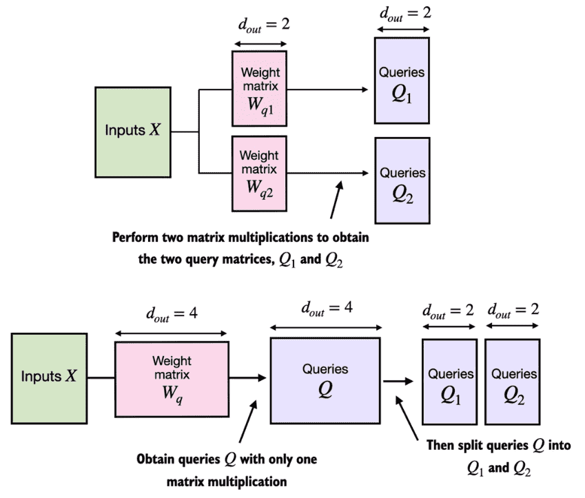
Figure 3.26 In the MultiheadAttentionWrapper class with two attention heads, we initialized two weight matrices \(W_{q1}\) and \(W_{q2}\) and computed two query matrices Q1 and Q2 as illustrated at the top of this figure. In the MultiheadAttention class, we initialize one larger weight matrix \(W_q\) , only perform one matrix multiplication with the inputs to obtain a query matrix Q, and then split the query matrix into Q1 and Q2 as shown at the bottom of this figure. We do the same for the keys and values, which are not shown to reduce visual clutter.
使用示例
torch.manual_seed(123)
batch_size, context_length, d_in = batch.shape
d_out = 2
mha = MultiHeadAttention(d_in, d_out, context_length, 0.0, num_heads=2)
context_vecs = mha(batch)
print("context_vecs.shape:", context_vecs.shape)
# context_vecs.shape: torch.Size([2, 6, 2])
print(context_vecs)
# tensor([[[0.3190, 0.4858],
#          [0.2943, 0.3897],
#          [0.2856, 0.3593],
#          [0.2693, 0.3873],
#          [0.2639, 0.3928],
#          [0.2575, 0.4028]],
#         [[0.3190, 0.4858],
#          [0.2943, 0.3897],
#          [0.2856, 0.3593],
#          [0.2693, 0.3873],
#          [0.2639, 0.3928],
#          [0.2575, 0.4028]]], grad_fn=<ViewBackward0>)
3.7 Summary
Attention mechanisms transform input elements into enhanced context vector representations that incorporate(包含,使合并) information about all inputs.
A self-attention mechanism computes the context vector representation as a weighted sum over the inputs.
In a simplified attention mechanism, the attention weights are computed via dot products.
A dot product is just a concise way of multiplying two vectors element-wise and then summing the products.
Matrix multiplications, while not strictly required, help us to implement computations more efficiently and compactly by replacing nested for-loops.
In self-attention mechanisms that are used in LLMs, also called scaled-dot product attention, we include trainable weight matrices to compute intermediate transformations of the inputs: queries, values, and keys. When working with LLMs that read and generate text from left to right, we add a causal attention mask to prevent the LLM from accessing future tokens.
Next to causal attention masks to zero out attention weights, we can also add a dropout mask to reduce overfitting in LLMs.
The attention modules in transformer-based LLMs involve multiple instances of causal attention, which is called multi-head attention.
We can create a multi-head attention module by stacking(堆叠) multiple instances of causal attention modules.
A more efficient way of creating multi-head attention modules involves batched matrix multiplications.
4 Implementing a GPT model from Scratch To Generate Text
Coding a GPT-like large language model (LLM) that can be trained to generate human-like text
Normalizing layer activations to stabilize neural network training
Adding shortcut connections in deep neural networks to train models more effectively
Implementing transformer blocks to create GPT models of various sizes
Computing the number of parameters and storage requirements of GPT models
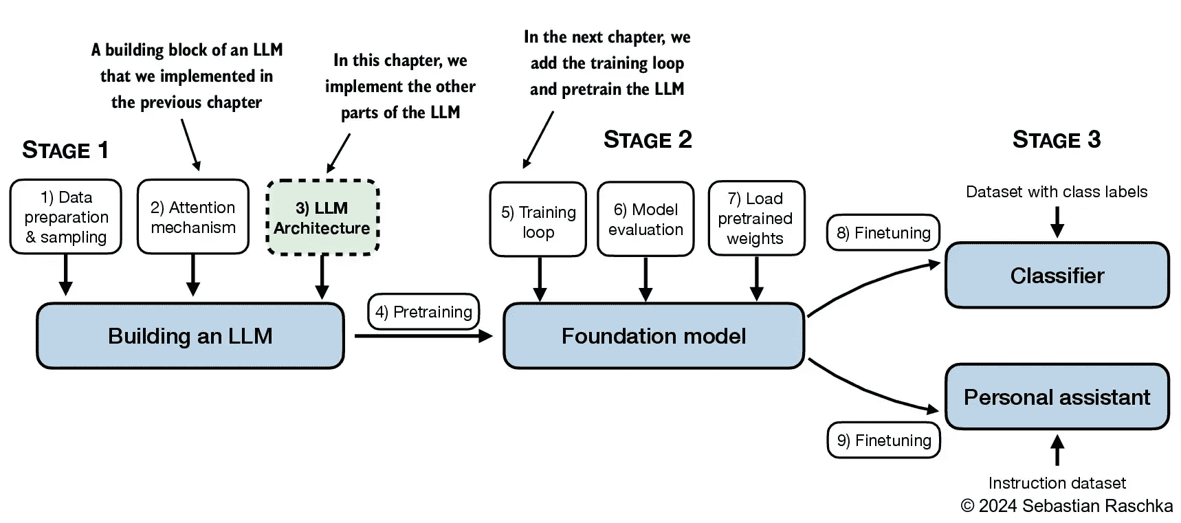
Figure 4.1 A mental model of the three main stages of coding an LLM, pretraining the LLM on a general text dataset, and finetuning it on a labeled dataset. This chapter focuses on implementing the LLM architecture, which we will train in the next chapter.
4.1 Coding an LLM architecture
In previous chapters, we used small embedding dimensions for token inputs and outputs for ease of illustration, ensuring they fit on a single page
In this chapter, we consider embedding and model sizes akin to a small GPT-2 model
We’ll specifically code the architecture of the smallest GPT-2 model (124 million parameters)
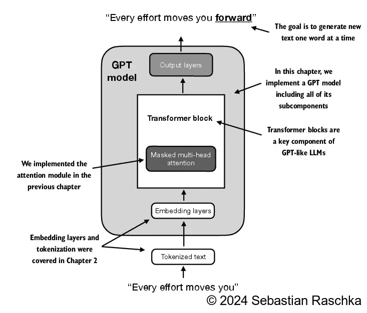
Figure 4.2 A mental model of a GPT model. Next to the embedding layers, it consists of one or more transformer blocks containing the masked multi-head attention module we implemented in the previous chapter.
configuration of the small GPT-2 model:
GPT_CONFIG_124M = {
    "vocab_size": 50257,        # Vocabulary size
    "context_length": 1024,     # Context length
    "emb_dim": 768,             # Embedding dimension
    "n_heads": 12,              # Number of attention heads
    "n_layers": 12,             # Number of layers
    "drop_rate": 0.1,           # Dropout rate
    "qkv_bias": False           # Query-Key-Value bias
}
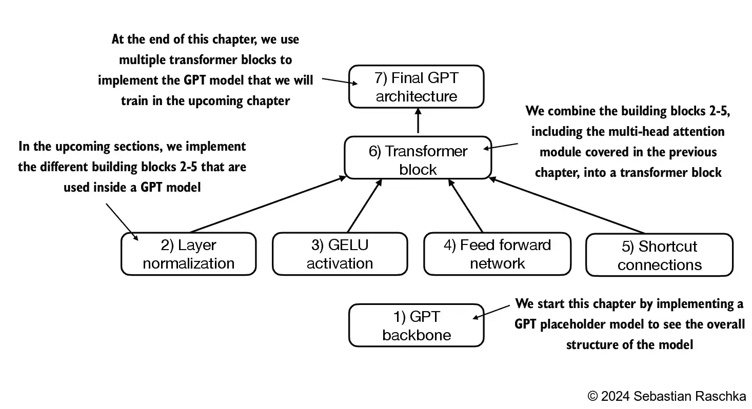
Figure 4.3 A mental model outlining the order in which we code the GPT architecture. In this chapter, we will start with the GPT backbone, a placeholder architecture, before we get to the individual core pieces and eventually assemble them in a transformer block for the final GPT architecture.
import torch
import torch.nn as nn


class DummyGPTModel(nn.Module):
    def __init__(self, cfg):
        super().__init__()
        self.tok_emb = nn.Embedding(cfg["vocab_size"], cfg["emb_dim"])
        self.pos_emb = nn.Embedding(cfg["context_length"], cfg["emb_dim"])
        self.drop_emb = nn.Dropout(cfg["drop_rate"])

        # Use a placeholder for TransformerBlock
        self.trf_blocks = nn.Sequential(
            *[DummyTransformerBlock(cfg) for _ in range(cfg["n_layers"])])

        # Use a placeholder for LayerNorm
        self.final_norm = DummyLayerNorm(cfg["emb_dim"])
        self.out_head = nn.Linear(
            cfg["emb_dim"], cfg["vocab_size"], bias=False
        )

    def forward(self, in_idx):
        batch_size, seq_len = in_idx.shape
        tok_embeds = self.tok_emb(in_idx)
        pos_embeds = self.pos_emb(torch.arange(seq_len, device=in_idx.device))
        x = tok_embeds + pos_embeds
        x = self.drop_emb(x)
        x = self.trf_blocks(x)
        x = self.final_norm(x)
        logits = self.out_head(x)
        return logits


class DummyTransformerBlock(nn.Module):
    def __init__(self, cfg):
        super().__init__()
        # A simple placeholder

    def forward(self, x):
        # This block does nothing and just returns its input.
        return x


class DummyLayerNorm(nn.Module):
    def __init__(self, normalized_shape, eps=1e-5):
        super().__init__()
        # The parameters here are just to mimic the LayerNorm interface.

    def forward(self, x):
        # This layer does nothing and just returns its input.
        return x
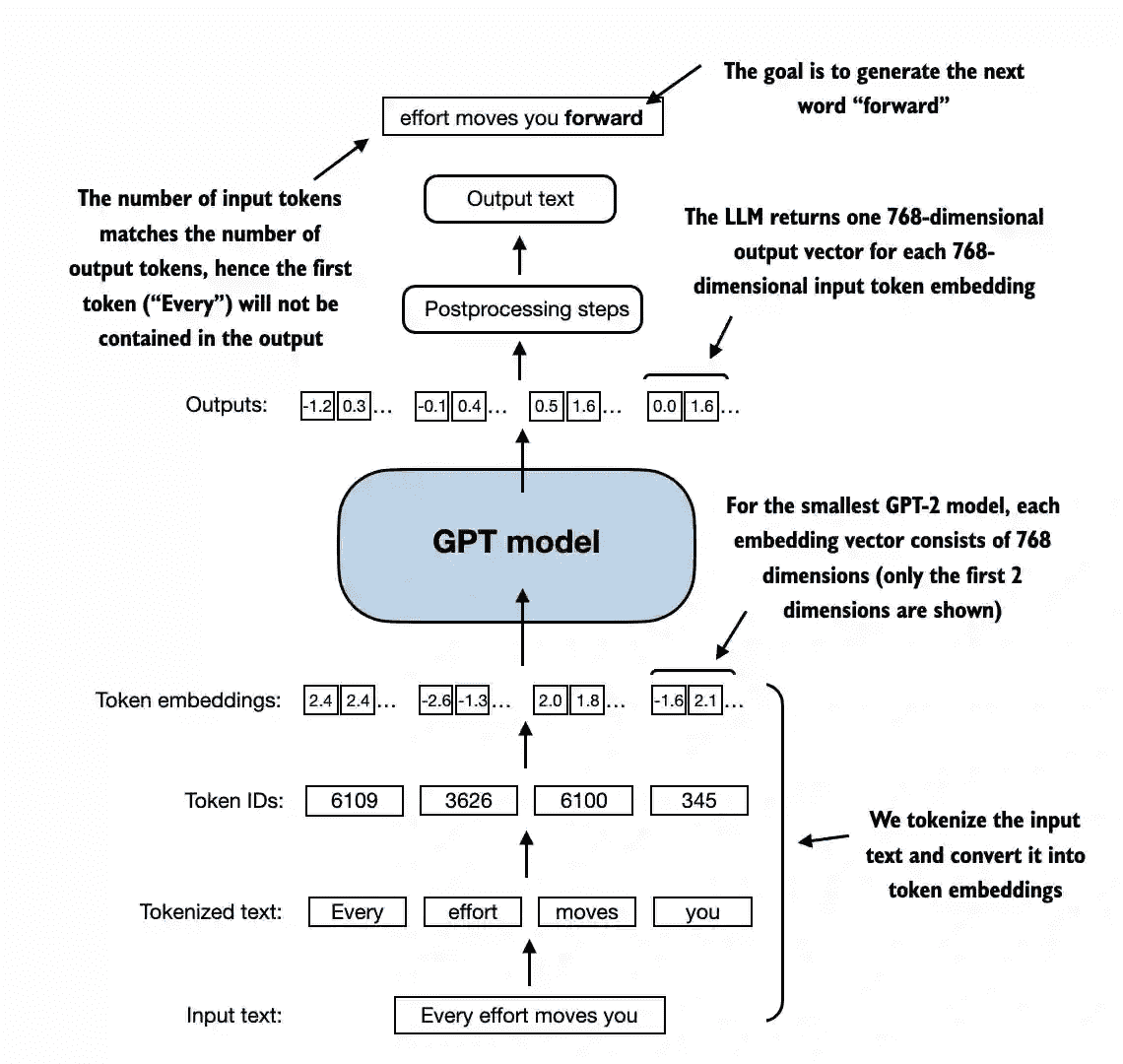
Figure 4.4 A big-picture overview showing how the input data is tokenized, embedded, and fed to the GPT model. Note that in our DummyGPTClass coded earlier, the token embedding is handled inside the GPT model. In LLMs, the embedded input token dimension typically matches the output dimension. The output embeddings here represent the context vectors we discussed in chapter 3.
import tiktoken
tokenizer = tiktoken.get_encoding("gpt2")
batch = []
txt1 = "Every effort moves you"
txt2 = "Every day holds a"
batch.append(torch.tensor(tokenizer.encode(txt1)))
batch.append(torch.tensor(tokenizer.encode(txt2)))
batch = torch.stack(batch, dim=0)
print(batch)
# tensor([[ 6109,  3626,  6100,   345], #A
#         [ 6109,  1110,  6622,   257]])

torch.manual_seed(123)
model = DummyGPTModel(GPT_CONFIG_124M)
logits = model(batch)
print("Output shape:", logits.shape)
print(logits)
# Output shape: torch.Size([2, 4, 50257])
# tensor([[[-1.2034,  0.3201, -0.7130,  ..., -1.5548, -0.2390, -0.4667],
#          [-0.1192,  0.4539, -0.4432,  ...,  0.2392,  1.3469,  1.2430],
#          [ 0.5307,  1.6720, -0.4695,  ...,  1.1966,  0.0111,  0.5835],
#          [ 0.0139,  1.6755, -0.3388,  ...,  1.1586, -0.0435, -1.0400]],
#         [[-1.0908,  0.1798, -0.9484,  ..., -1.6047,  0.2439, -0.4530],
#          [-0.7860,  0.5581, -0.0610,  ...,  0.4835, -0.0077,  1.6621],
#          [ 0.3567,  1.2698, -0.6398,  ..., -0.0162, -0.1296,  0.3717],
#          [-0.2407, -0.7349, -0.5102,  ...,  2.0057, -0.3694,  0.1814]]],
#        grad_fn=<UnsafeViewBackward0>)
4.2 Normalizing activations with layer normalization
Training deep neural networks with many layers can sometimes prove challenging due to issues like vanishing or exploding gradients.
These issues lead to unstable training dynamics and make it difficult for the network to effectively adjust its weights, which means the learning process struggles to find a set of parameters (weights) for the neural network that minimizes the loss function.
In other words, the network has difficulty learning the underlying patterns in the data to a degree that would allow it to make accurate predictions or decisions.
The main idea behind layer normalization is to adjust the
activations (outputs)of a neural network layer to have a mean of 0 and a variance of 1, also known asunit variance.
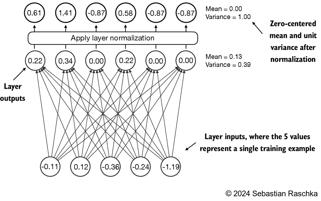
Figure 4.5 An illustration of layer normalization where the 5 layer outputs, also called activations, are normalized such that they have a zero mean and variance of 1.
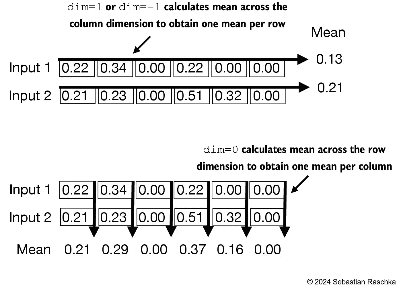
Figure 4.6 An illustration of the dim parameter when calculating the mean of a tensor. For instance,if we have a 2D tensor(matrix) with dimensions[rows, columns], using dim=0 will perform the operation across rows (vertically, as shown at the bottom), resulting in an output that aggregates the data for each column. Using dim=1 or dim=-1 will perform the operation across columns (horizontally, as shown at the top), resulting in an output aggregating the data for each row.
# 归一化L2(欧几里德范数归一)
class LayerNorm(nn.Module):
    def __init__(self, emb_dim):
        super().__init__()
        self.eps = 1e-5
        self.scale = nn.Parameter(torch.ones(emb_dim))
        self.shift = nn.Parameter(torch.zeros(emb_dim))

    def forward(self, x):
        mean = x.mean(dim=-1, keepdim=True)
        var = x.var(dim=-1, keepdim=True, unbiased=False)
        norm_x = (x - mean) / torch.sqrt(var + self.eps)
        return self.scale * norm_x + self.shift
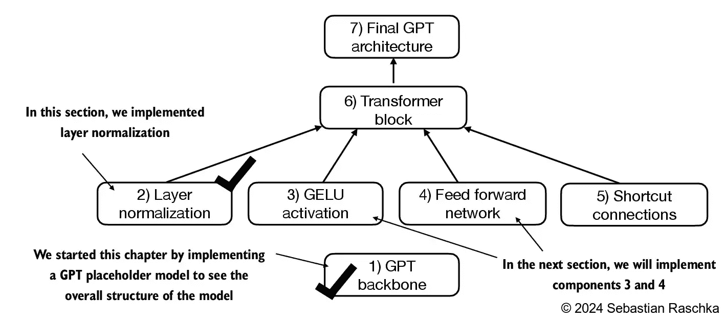
Figure 4.7 A mental model listing the different building blocks we implement in this chapter to assemble the GPT architecture.
4.3 Implementing a feed forward network with GELU activations
主要讲了GELU的实现和特点
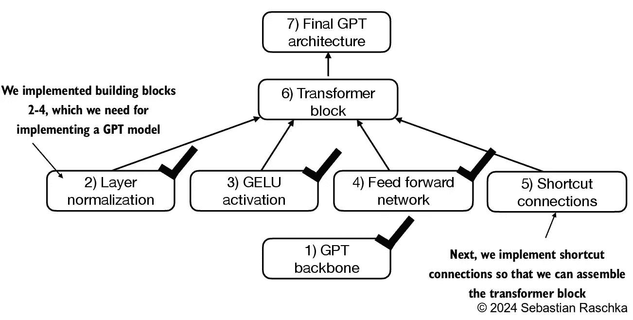
Figure 4.11 A mental model showing the topics we cover in this chapter, with the black checkmarks indicating those that we have already covered.
4.4 Adding shortcut connections
shortcut connections, also known asskip or residual connections.Originally,
shortcut connectionswere proposed for deep networks in computer vision (specifically, in residual networks) to mitigate the challenge of vanishing gradients.The vanishing gradient problem refers to the issue where gradients (which guide weight updates during training) become progressively smaller as they propagate backward through the layers, making it difficult to effectively train earlier layers
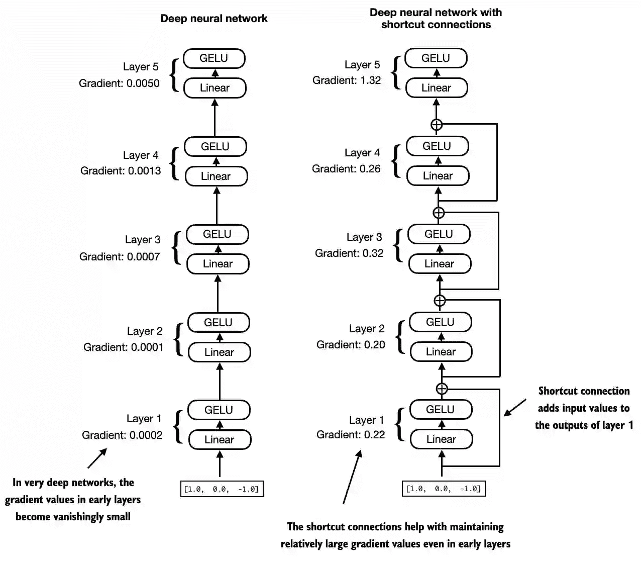
Figure 4.12 A comparison between a deep neural network consisting of 5 layers without (on the left) and with shortcut connections (on the right). Shortcut connections involve adding the inputs of a layer to its outputs, effectively creating an alternate path that bypasses certain layers. The gradient illustrated in Figure 1.1 denotes the mean absolute gradient at each layer, which we will compute in the code example that follows.
class ExampleDeepNeuralNetwork(nn.Module):
    def __init__(self, layer_sizes, use_shortcut):
        super().__init__()
        self.use_shortcut = use_shortcut
        self.layers = nn.ModuleList([
            nn.Sequential(nn.Linear(layer_sizes[0], layer_sizes[1]), GELU()),
            nn.Sequential(nn.Linear(layer_sizes[1], layer_sizes[2]), GELU()),
            nn.Sequential(nn.Linear(layer_sizes[2], layer_sizes[3]), GELU()),
            nn.Sequential(nn.Linear(layer_sizes[3], layer_sizes[4]), GELU()),
            nn.Sequential(nn.Linear(layer_sizes[4], layer_sizes[5]), GELU())
        ])

    def forward(self, x):
        for layer in self.layers:
            # Compute the output of the current layer
            layer_output = layer(x)
            # Check if shortcut can be applied
            if self.use_shortcut and x.shape == layer_output.shape:
                x = x + layer_output
            else:
                x = layer_output
        return x

def print_gradients(model, x):
    # Forward pass
    output = model(x)
    target = torch.tensor([[0.]])

    # Calculate loss based on how close the target
    # and output are
    loss = nn.MSELoss()
    loss = loss(output, target)

    # Backward pass to calculate the gradients
    loss.backward()

    for name, param in model.named_parameters():
        if 'weight' in name:
            # Print the mean absolute gradient of the weights
            print(f"{name} has gradient mean of {param.grad.abs().mean().item()}")
print the gradient values without shortcut connections:
layer_sizes = [3, 3, 3, 3, 3, 1]

sample_input = torch.tensor([[1., 0., -1.]])

torch.manual_seed(123)
model_without_shortcut = ExampleDeepNeuralNetwork(
    layer_sizes, use_shortcut=False
)
print_gradients(model_without_shortcut, sample_input)

# 输出 ==>
# layers.0.0.weight has gradient mean of 0.00020173587836325169
# layers.1.0.weight has gradient mean of 0.0001201116101583466
# layers.2.0.weight has gradient mean of 0.0007152041653171182
# layers.3.0.weight has gradient mean of 0.001398873864673078
# layers.4.0.weight has gradient mean of 0.005049646366387606
print the gradient values with shortcut connections:
torch.manual_seed(123)
model_with_shortcut = ExampleDeepNeuralNetwork(
    layer_sizes, use_shortcut=True
)
print_gradients(model_with_shortcut, sample_input)
# 输出 ==>
# layers.0.0.weight has gradient mean of 0.22169792652130127
# layers.1.0.weight has gradient mean of 0.20694105327129364
# layers.2.0.weight has gradient mean of 0.32896995544433594
# layers.3.0.weight has gradient mean of 0.2665732502937317
# layers.4.0.weight has gradient mean of 1.3258541822433472
4.5 Connecting attention and linear layers in a transformer block
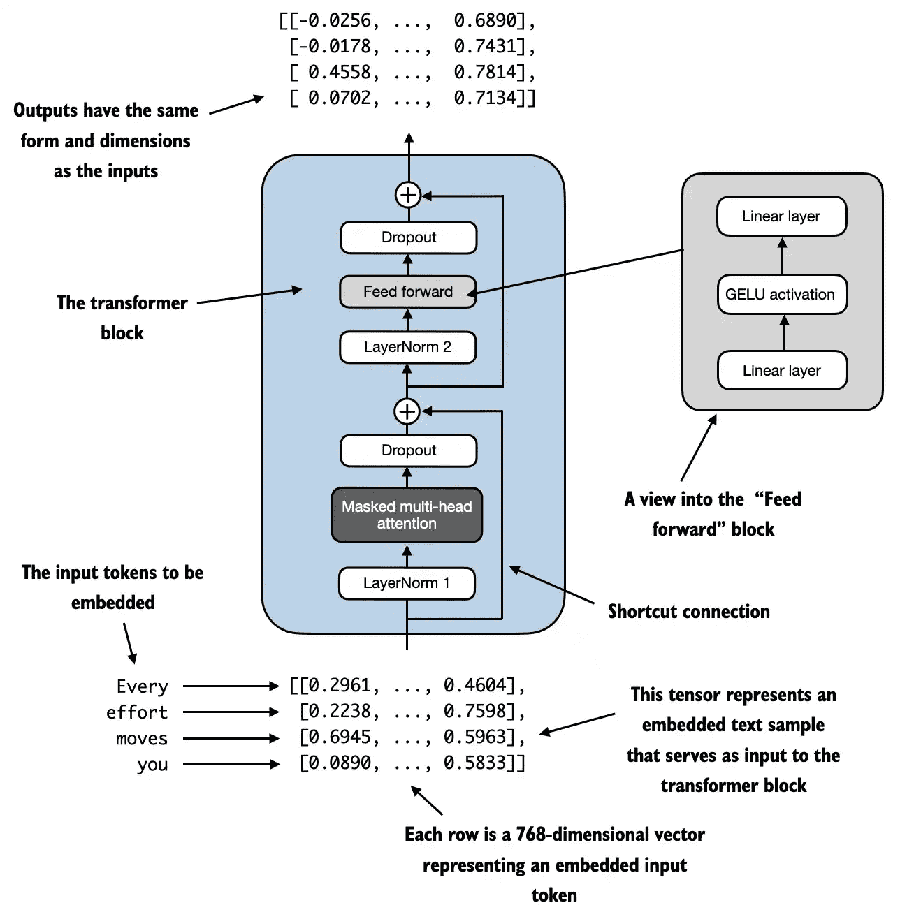
Figure 4.13 An illustration of a transformer block. The bottom of the diagram shows input tokens that have been embedded into 768-dimensional vectors. Each row corresponds to one token’s vector representation. The outputs of the transformer block are vectors of the same dimension as the input, which can then be fed into subsequent layers in an LLM.
The idea is that the self-attention mechanism in the multi-head attention block identifies and analyzes relationships between elements in the input sequence.
In contrast, the feed forward network modifies the data individually at each position.
This combination not only enables a more nuanced(细微差别) understanding and processing of the input but also enhances the model’s overall capacity for handling complex data patterns.
【组合的意义 fromGPT】自注意力机制提供全局信息:通过捕捉序列中元素之间的关系,让模型理解上下文和结构的复杂性。前馈网络强化局部信息:对每个位置进行特定的非线性变换,提升其独立特征表达。协同效果:这种组合让模型既能捕捉全局模式,又能处理局部细节,从而在面对复杂数据模式时表现出更强的处理能力。【例】句子翻译任务:自注意力机制帮助模型理解句子结构和词语之间的关系;前馈网络对每个单词的特定信息进行调整和优化,从而生成更准确的翻译。
from previous_chapters import MultiHeadAttention

class TransformerBlock(nn.Module):
    def __init__(self, cfg):
        super().__init__()
        self.att = MultiHeadAttention(
            d_in=cfg["emb_dim"],
            d_out=cfg["emb_dim"],
            context_length=cfg["context_length"],
            num_heads=cfg["n_heads"],
            dropout=cfg["drop_rate"],
            qkv_bias=cfg["qkv_bias"])
        self.ff = FeedForward(cfg)
        self.norm1 = LayerNorm(cfg["emb_dim"])
        self.norm2 = LayerNorm(cfg["emb_dim"])
        self.drop_shortcut = nn.Dropout(cfg["drop_rate"])

    def forward(self, x):
        # Shortcut connection for attention block
        shortcut = x
        x = self.norm1(x)
        x = self.att(x)  # Shape [batch_size, num_tokens, emb_size]
        x = self.drop_shortcut(x)
        x = x + shortcut  # Add the original input back

        # Shortcut connection for feed forward block
        shortcut = x
        x = self.norm2(x)
        x = self.ff(x)
        x = self.drop_shortcut(x)
        x = x + shortcut  # Add the original input back

        return x
输入&输出形状相同,是一个关键设计
The preservation of shape throughout the transformer block architecture is not incidental but a crucial aspect of its design.
This design enables its effective application across a wide range of sequence-to-sequence tasks, where each output vector directly corresponds to an input vector, maintaining a one-to-one relationship.
However, the output is a context vector that encapsulates information from the entire input sequence, as we learned in chapter 3.
This means that while the physical dimensions of the sequence (length and feature size) remain unchanged as it passes through the transformer block, the content of each output vector is re-encoded to integrate contextual information from across the entire input sequence.
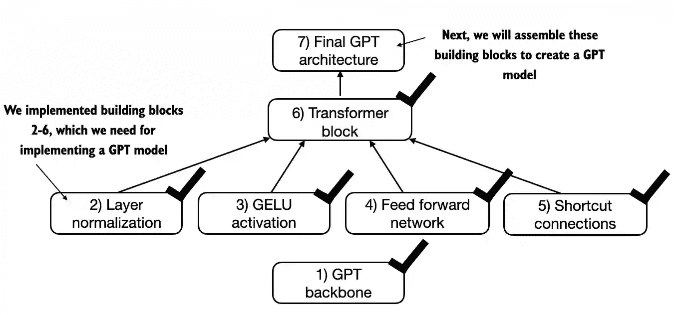
Figure 4.14 A mental model of the different concepts we have implemented in this chapter so far.
4.6 Coding the GPT model
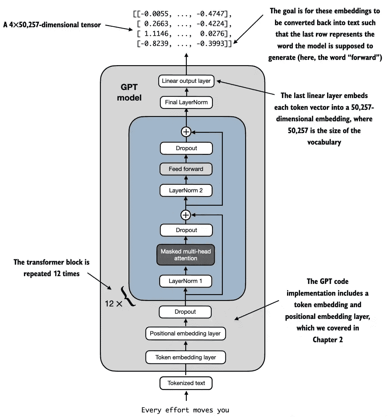
Figure 4.15 An overview of the GPT model architecture. This figure illustrates the flow of data through the GPT model. Starting from the bottom, tokenized text is first converted into token embeddings, which are then augmented with positional embeddings. This combined information forms a tensor that is passed through a series of transformer blocks shown in the center (each containing multi-head attention and feed forward neural network layers with dropout and layer normalization), which are stacked on top of each other and repeated 12 times.
the transformer block is repeated many times throughout a GPT model architecture.
In the case of the 124 million parameter GPT-2 model, it’s repeated 12 times
In the case of the largest GPT-2 model with 1,542 million parameters, this transformer block is repeated 36 times.
class GPTModel(nn.Module):
    def __init__(self, cfg):
        super().__init__()
        self.tok_emb = nn.Embedding(cfg["vocab_size"], cfg["emb_dim"])
        self.pos_emb = nn.Embedding(cfg["context_length"], cfg["emb_dim"])
        self.drop_emb = nn.Dropout(cfg["drop_rate"])

        self.trf_blocks = nn.Sequential(
            *[TransformerBlock(cfg) for _ in range(cfg["n_layers"])])

        self.final_norm = LayerNorm(cfg["emb_dim"])
        self.out_head = nn.Linear(
            cfg["emb_dim"], cfg["vocab_size"], bias=False
        )

    def forward(self, in_idx):
        batch_size, seq_len = in_idx.shape
        tok_embeds = self.tok_emb(in_idx)
        pos_embeds = self.pos_emb(torch.arange(seq_len, device=in_idx.device))
        x = tok_embeds + pos_embeds  # Shape [batch_size, num_tokens, emb_size]
        x = self.drop_emb(x)
        x = self.trf_blocks(x)
        x = self.final_norm(x)
        logits = self.out_head(x)
        return logits
请求:
torch.manual_seed(123)
model = GPTModel(GPT_CONFIG_124M)

out = model(batch)
print("Input batch:\n", batch)
print("\nOutput shape:", out.shape)
print(out)

# 输出
# Input batch:
#  tensor([[6109, 3626, 6100,  345],
#         [6109, 1110, 6622,  257]])

# Output shape: torch.Size([2, 4, 50257])
# tensor([[[ 0.3613,  0.4222, -0.0711,  ...,  0.3483,  0.4661, -0.2838],
#          [-0.1792, -0.5660, -0.9485,  ...,  0.0477,  0.5181, -0.3168],
#          [ 0.7120,  0.0332,  0.1085,  ...,  0.1018, -0.4327, -0.2553],
#          [-1.0076,  0.3418, -0.1190,  ...,  0.7195,  0.4023,  0.0532]],

#         [[-0.2564,  0.0900,  0.0335,  ...,  0.2659,  0.4454, -0.6806],
#          [ 0.1230,  0.3653, -0.2074,  ...,  0.7705,  0.2710,  0.2246],
#          [ 1.0558,  1.0318, -0.2800,  ...,  0.6936,  0.3205, -0.3178],
#          [-0.1565,  0.3926,  0.3288,  ...,  1.2630, -0.1858,  0.0388]]],
#        grad_fn=<UnsafeViewBackward0>)
参看参数总数:
total_params = sum(p.numel() for p in model.parameters())
print(f"Total number of parameters: {total_params:,}")

# 输出
Total number of parameters: 163,009,536
# 疑问
为啥不是 GPT2 论文说的 124M 呢?
备注
In the original GPT-2 paper, the researchers applied weight tying , which means that they reused the token embedding layer (tok_emb) as the output layer, which means setting self.out_head.weight = self.tok_emb.weight . The token embedding and output layers are very large due to the number of rows for the 50,257 in the tokenizer’s vocabulary. Weight tying reduces the overall memory footprint and computational complexity of the model. 具体参见 WeightTying
去除GPT2重用的参数:
total_params_gpt2 =  total_params - sum(p.numel() for p in model.out_head.parameters())
print(f"Number of trainable parameters considering weight tying: {total_params_gpt2:,}")

# 输出
Number of trainable parameters considering weight tying: 124,412,160
内存占用:
# Calculate the total size in bytes (assuming float32, 4 bytes per parameter)
total_size_bytes = total_params * 4

# Convert to megabytes
total_size_mb = total_size_bytes / (1024 * 1024)

print(f"Total size of the model: {total_size_mb:.2f} MB")
# 输出
Total size of the model: 621.83 MB
Exercise:
- **GPT2-small** (the 124M configuration we already implemented):
    - "emb_dim" = 768
    - "n_layers" = 12
    - "n_heads" = 12

- **GPT2-medium:**
    - "emb_dim" = 1024
    - "n_layers" = 24
    - "n_heads" = 16

- **GPT2-large:**
    - "emb_dim" = 1280
    - "n_layers" = 36
    - "n_heads" = 20

- **GPT2-XL:**
    - "emb_dim" = 1600
    - "n_layers" = 48
    - "n_heads" = 25
4.7 Generating text
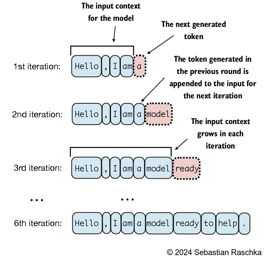
Figure 4.16 This diagram illustrates the step-by-step process by which an LLM generates text, one token at a time. Starting with an initial input context (“Hello, I am”), the model predicts a subsequent token during each iteration, appending it to the input context for the next round of prediction. As shown, the first iteration adds “a”, the second “model”, and the third “ready”, progressively building the sentence.
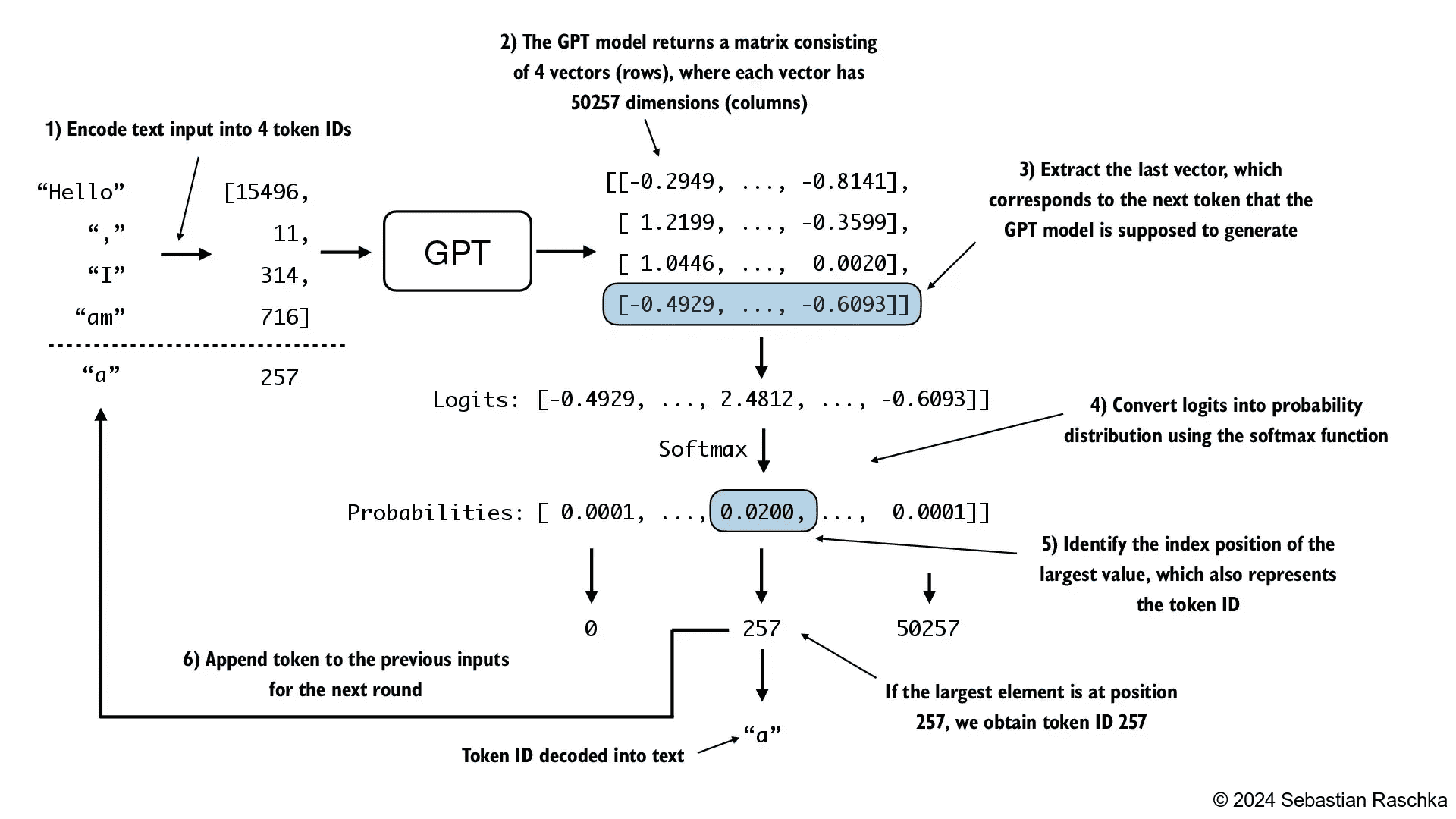
Figure 4.17 details the mechanics of text generation in a GPT model by showing a single iteration in the token generation process. The process begins by encoding the input text into token IDs, which are then fed into the GPT model. The outputs of the model are then converted back into text and appended to the original input text.
def generate_text_simple(model, idx, max_new_tokens, context_size):
    # idx is (batch, n_tokens) array of indices in the current context
    for _ in range(max_new_tokens):

        # Crop current context if it exceeds the supported context size
        # E.g., if LLM supports only 5 tokens, and the context size is 10
        # then only the last 5 tokens are used as context
        idx_cond = idx[:, -context_size:]

        # Get the predictions
        with torch.no_grad():
            logits = model(idx_cond)

        # Focus only on the last time step
        # (batch, n_tokens, vocab_size) becomes (batch, vocab_size)
        logits = logits[:, -1, :]

        # Apply softmax to get probabilities
        probas = torch.softmax(logits, dim=-1)  # (batch, vocab_size)

        # Get the idx of the vocab entry with the highest probability value
        idx_next = torch.argmax(probas, dim=-1, keepdim=True)  # (batch, 1)

        # Append sampled index to the running sequence
        idx = torch.cat((idx, idx_next), dim=1)  # (batch, n_tokens+1)

    return idx
备注
其实这儿不用执行 torch.softmax 直接执行 torch.softmax 可以得到同样的结果。we coded the conversion to illustrate the full process of transforming logits to probabilities, which can add additional intuition, such as that the model generates the most likely next token, which is known as greedy decoding. In the next chapter, when we will implement the GPT training code, we will also introduce additional sampling techniques where we modify the softmax outputs such that the model doesn’t always select the most likely token, which introduces variability and creativity in the generated text.
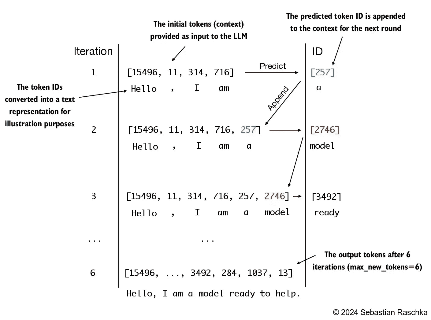
Figure 4.18 An illustration showing six iterations of a token prediction cycle, where the model takes a sequence of initial token IDs as input, predicts the next token, and appends this token to the input sequence for the next iteration. (The token IDs are also translated into their corresponding text for better understanding.)
准备数据:
start_context = "Hello, I am"

encoded = tokenizer.encode(start_context)
print("encoded:", encoded)

encoded_tensor = torch.tensor(encoded).unsqueeze(0)
print("encoded_tensor.shape:", encoded_tensor.shape)
# 输出
# encoded: [15496, 11, 314, 716]
# encoded_tensor.shape: torch.Size([1, 4])
put the model into .eval() mode, which disables random components like dropout, which are only used during training:
model.eval() # disable dropout

out = generate_text_simple(
    model=model,
    idx=encoded_tensor,
    max_new_tokens=6,
    context_size=GPT_CONFIG_124M["context_length"]
)

print("Output:", out)
print("Output length:", len(out[0]))
# 输出
# Output: tensor([[15496,    11,   314,   716, 27018, 24086, 47843, 30961, 42348,  7267]])
# Output length: 10
Remove batch dimension and convert back into text:
decoded_text = tokenizer.decode(out.squeeze(0).tolist())
print(decoded_text)
# 输出(未训练的)
# Hello, I am Featureiman Byeswickattribute argue
4.8 Summary
Layer normalization stabilizes training by ensuring that each layer’s outputs have a consistent mean and variance.
Shortcut connections are connections that skip one or more layers by feeding the output of one layer directly to a deeper layer, which helps mitigate the vanishing gradient problem when training deep neural networks, such as LLMs.
Transformer blocks are a core structural component of GPT models, combining
masked multi-head attention moduleswithfully connected feed-forward networksthat use the GELU activation function.GPT models are LLMs with many repeated transformer blocks that have millions to billions of parameters.
GPT models come in various sizes, for example, 124 million, and 1542 million parameters, which we can implement with the same GPTModel Python class.
The text generation capability of a GPT-like LLM involves decoding output tensors into human-readable text by sequentially predicting one token at a time based on a given input context.
Without training, a GPT model generates incoherent text, which underscores the importance of model training for coherent text generation, which is the topic of subsequent chapters.
import torch
import torch.nn as nn


class LayerNorm(nn.Module):
    def __init__(self, emb_dim):
        super().__init__()
        self.eps = 1e-5
        self.scale = nn.Parameter(torch.ones(emb_dim))
        self.shift = nn.Parameter(torch.zeros(emb_dim))

    def forward(self, x):
        mean = x.mean(dim=-1, keepdim=True)
        var = x.var(dim=-1, keepdim=True, unbiased=False)
        norm_x = (x - mean) / torch.sqrt(var + self.eps)
        return self.scale * norm_x + self.shift


class GELU(nn.Module):
    def __init__(self):
        super().__init__()

    def forward(self, x):
        return 0.5 * x * (1 + torch.tanh(
            torch.sqrt(torch.tensor(2.0 / torch.pi)) *
            (x + 0.044715 * torch.pow(x, 3))
        ))

class FeedForward(nn.Module):
    def __init__(self, cfg):
        super().__init__()
        self.layers = nn.Sequential(
            nn.Linear(cfg["emb_dim"], 4 * cfg["emb_dim"]),
            GELU(),
            nn.Linear(4 * cfg["emb_dim"], cfg["emb_dim"]),
        )

    def forward(self, x):
        return self.layers(x)


class MultiHeadAttention(nn.Module):
    def __init__(self, d_in, d_out, context_length, dropout, num_heads, qkv_bias=False):
        super().__init__()
        assert d_out % num_heads == 0, "d_out must be divisible by num_heads"

        self.d_out = d_out
        self.num_heads = num_heads
        self.head_dim = d_out // num_heads  # Reduce the projection dim to match desired output dim

        self.W_query = nn.Linear(d_in, d_out, bias=qkv_bias)
        self.W_key = nn.Linear(d_in, d_out, bias=qkv_bias)
        self.W_value = nn.Linear(d_in, d_out, bias=qkv_bias)
        self.out_proj = nn.Linear(d_out, d_out)  # Linear layer to combine head outputs
        self.dropout = nn.Dropout(dropout)
        self.register_buffer('mask', torch.triu(torch.ones(context_length, context_length), diagonal=1))

    def forward(self, x):
        b, num_tokens, d_in = x.shape

        keys = self.W_key(x)  # Shape: (b, num_tokens, d_out)
        queries = self.W_query(x)
        values = self.W_value(x)

        # We implicitly split the matrix by adding a `num_heads` dimension
        # Unroll last dim: (b, num_tokens, d_out) -> (b, num_tokens, num_heads, head_dim)
        keys = keys.view(b, num_tokens, self.num_heads, self.head_dim)
        values = values.view(b, num_tokens, self.num_heads, self.head_dim)
        queries = queries.view(b, num_tokens, self.num_heads, self.head_dim)

        # Transpose: (b, num_tokens, num_heads, head_dim) -> (b, num_heads, num_tokens, head_dim)
        keys = keys.transpose(1, 2)
        queries = queries.transpose(1, 2)
        values = values.transpose(1, 2)

        # Compute scaled dot-product attention (aka self-attention) with a causal mask
        attn_scores = queries @ keys.transpose(2, 3)  # Dot product for each head

        # Original mask truncated to the number of tokens and converted to boolean
        mask_bool = self.mask.bool()[:num_tokens, :num_tokens]

        # Use the mask to fill attention scores
        attn_scores.masked_fill_(mask_bool, -torch.inf)

        attn_weights = torch.softmax(attn_scores / keys.shape[-1]**0.5, dim=-1)
        attn_weights = self.dropout(attn_weights)

        # Shape: (b, num_tokens, num_heads, head_dim)
        context_vec = (attn_weights @ values).transpose(1, 2)

        # Combine heads, where self.d_out = self.num_heads * self.head_dim
        context_vec = context_vec.contiguous().view(b, num_tokens, self.d_out)
        context_vec = self.out_proj(context_vec)  # optional projection

        return context_vec


class TransformerBlock(nn.Module):
    def __init__(self, cfg):
        super().__init__()
        self.att = MultiHeadAttention(
            d_in=cfg["emb_dim"],
            d_out=cfg["emb_dim"],
            context_length=cfg["context_length"],
            num_heads=cfg["n_heads"],
            dropout=cfg["drop_rate"],
            qkv_bias=cfg["qkv_bias"])
        self.ff = FeedForward(cfg)
        self.norm1 = LayerNorm(cfg["emb_dim"])
        self.norm2 = LayerNorm(cfg["emb_dim"])
        self.drop_shortcut = nn.Dropout(cfg["drop_rate"])

    def forward(self, x):
        # Shortcut connection for attention block
        shortcut = x
        x = self.norm1(x)
        x = self.att(x)  # Shape [batch_size, num_tokens, emb_size]
        x = self.drop_shortcut(x)
        x = x + shortcut  # Add the original input back

        # Shortcut connection for feed forward block
        shortcut = x
        x = self.norm2(x)
        x = self.ff(x)
        x = self.drop_shortcut(x)
        x = x + shortcut  # Add the original input back

        return x

def generate_text_simple(model, idx, max_new_tokens, context_size):
    # idx is (batch, n_tokens) array of indices in the current context
    for _ in range(max_new_tokens):

        # Crop current context if it exceeds the supported context size
        # E.g., if LLM supports only 5 tokens, and the context size is 10
        # then only the last 5 tokens are used as context
        idx_cond = idx[:, -context_size:]

        # Get the predictions
        with torch.no_grad():
            logits = model(idx_cond)

        # Focus only on the last time step
        # (batch, n_tokens, vocab_size) becomes (batch, vocab_size)
        logits = logits[:, -1, :]

        # Apply softmax to get probabilities
        probas = torch.softmax(logits, dim=-1)  # (batch, vocab_size)

        # Get the idx of the vocab entry with the highest probability value
        idx_next = torch.argmax(probas, dim=-1, keepdim=True)  # (batch, 1)

        # Append sampled index to the running sequence
        idx = torch.cat((idx, idx_next), dim=1)  # (batch, n_tokens+1)

    return idx

class GPTModel(nn.Module):
    def __init__(self, cfg):
        super().__init__()
        self.tok_emb = nn.Embedding(cfg["vocab_size"], cfg["emb_dim"])
        self.pos_emb = nn.Embedding(cfg["context_length"], cfg["emb_dim"])
        self.drop_emb = nn.Dropout(cfg["drop_rate"])

        self.trf_blocks = nn.Sequential(
            *[TransformerBlock(cfg) for _ in range(cfg["n_layers"])])

        self.final_norm = LayerNorm(cfg["emb_dim"])
        self.out_head = nn.Linear(
            cfg["emb_dim"], cfg["vocab_size"], bias=False
        )

    def forward(self, in_idx):
        batch_size, seq_len = in_idx.shape
        tok_embeds = self.tok_emb(in_idx)
        pos_embeds = self.pos_emb(torch.arange(seq_len, device=in_idx.device))
        x = tok_embeds + pos_embeds  # Shape [batch_size, num_tokens, emb_size]
        x = self.drop_emb(x)
        x = self.trf_blocks(x)
        x = self.final_norm(x)
        logits = self.out_head(x)
        return logits

GPT_CONFIG_124M = {
    "vocab_size": 50257,    # Vocabulary size
    "context_length": 1024, # Context length
    "emb_dim": 768,         # Embedding dimension
    "n_heads": 12,          # Number of attention heads
    "n_layers": 12,         # Number of layers
    "drop_rate": 0.1,       # Dropout rate
    "qkv_bias": False       # Query-Key-Value bias
}

import tiktoken

tokenizer = tiktoken.get_encoding("gpt2")

start_context = "Hello, I am"
encoded = tokenizer.encode(start_context)
encoded_tensor = torch.tensor(encoded).unsqueeze(0)

torch.manual_seed(123)
model = GPTModel(GPT_CONFIG_124M)
model.eval() # disable dropout

out = generate_text_simple(
    model=model,
    idx=encoded_tensor,
    max_new_tokens=6,
    context_size=GPT_CONFIG_124M["context_length"]
)

decoded_text = tokenizer.decode(out.squeeze(0).tolist())
print(decoded_text)
5 Pretraining on Unlabeled Data
Computing the training and validation set losses to assess the quality of LLM-generated text during training
Implementing a training function and pretraining the LLM
Saving and loading model weights to continue training an LLM Loading pretrained weights from OpenAI
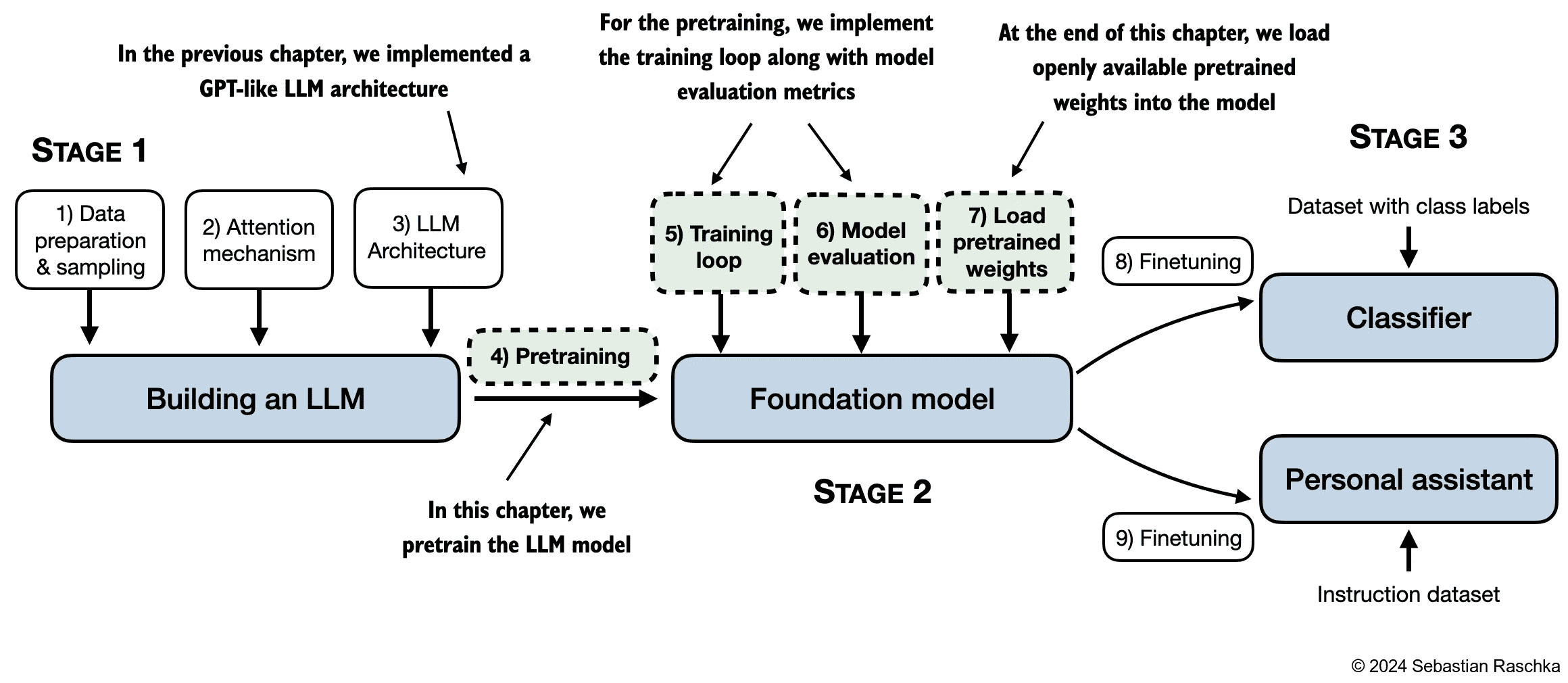
Figure 5.1 A mental model of the three main stages of coding an LLM, pretraining the LLM on a general text dataset and finetuning it on a labeled dataset. This chapter focuses on pretraining the LLM, which includes implementing the training code, evaluating the performance, and saving and loading model weights.
5.1 Evaluating generative text models
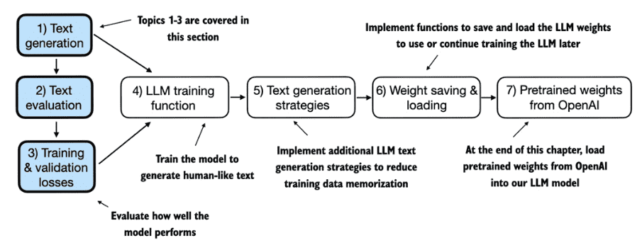
Figure 5.2 An overview of the topics covered in this chapter. We begin by recapping the text generation from the previous chapter and implementing basic model evaluation techniques that we can use during the pretraining stage.
5.1.1 Using GPT to generate text
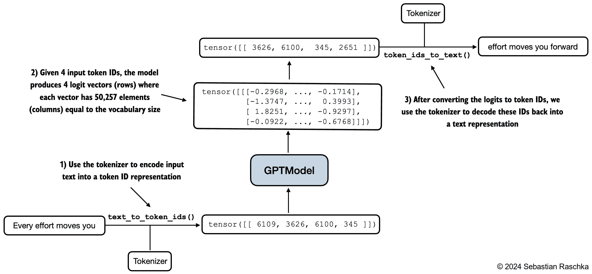
Figure 5.3 Generating text involves encoding text into token IDs that the LLM processes into logit vectors. The logit vectors are then converted back into token IDs, detokenized into a text representation.
Utility functions for text to token ID conversion
import tiktoken
from previous_chapters import generate_text_simple

def text_to_token_ids(text, tokenizer):
    encoded = tokenizer.encode(text, allowed_special={'<|endoftext|>'})
    encoded_tensor = torch.tensor(encoded).unsqueeze(0) # add batch dimension
    return encoded_tensor

def token_ids_to_text(token_ids, tokenizer):
    flat = token_ids.squeeze(0) # remove batch dimension
    return tokenizer.decode(flat.tolist())

start_context = "Every effort moves you"
tokenizer = tiktoken.get_encoding("gpt2")

token_ids = generate_text_simple(
    model=model,
    idx=text_to_token_ids(start_context, tokenizer),
    max_new_tokens=10,
    context_size=GPT_CONFIG_124M["context_length"]
)

print("Output text:\n", token_ids_to_text(token_ids, tokenizer))

# 输出
# Output text:
#  Every effort moves you rentingetic wasnم refres RexMeCHicular stren
5.1.2 Calculating the text generation loss
先回顾一下前面 how the data is loaded from chapter 2 and how the text is generated via the generate_text_simple function from chapter 4.
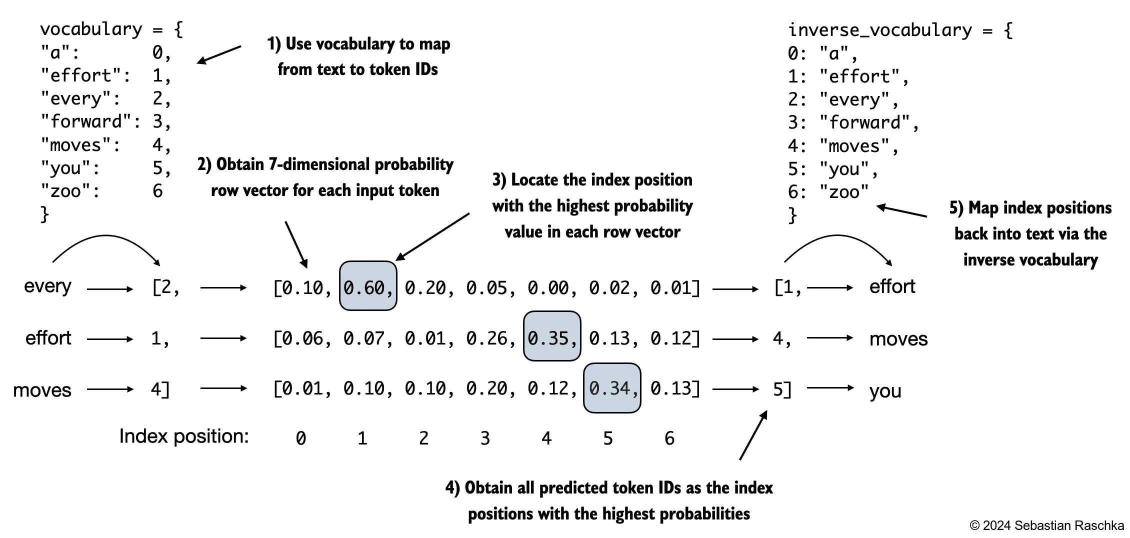
Figure 5.4 For each of the 3 input tokens, shown on the left, we compute a vector containing probability scores corresponding to each token in the vocabulary. The index position of the highest probability score in each vector represents the most likely next token ID. These token IDs associated with the highest probability scores are selected and mapped back into a text that represents the text generated by the model.
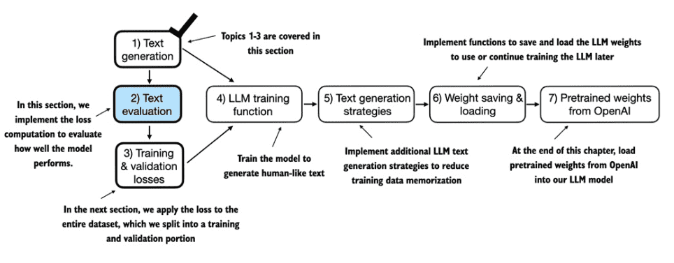
Figure 5.5 We now implement the text evaluation function in the remainder of this section. In the next section, we apply this evaluation function to the entire dataset we use for model training
输入&期望输出:
inputs = torch.tensor([[16833, 3626, 6100],   # ["every effort moves",
                       [40,    1107, 588]])   #  "I really like"]

targets = torch.tensor([[3626, 6100, 345  ],  # [" effort moves you",
                        [1107,  588, 11311]]) #  " really like chocolate"]
We feed the inputs into the model to calculate logit vectors for the two input examples, each comprising three tokens, and apply the softmax function to transform these logit values into probability scores:
with torch.no_grad():
    logits = model(inputs)

probas = torch.softmax(logits, dim=-1) # Probability of each token in vocabulary
print(probas.shape) # Shape: (batch_size, num_tokens, vocab_size)
# 输出
# torch.Size([2, 3, 50257])
by applying the argmax function to the probability scores to obtain the corresponding token IDs:
# 这儿得到的是模型的最终输出和token ID(当然现在还没训练,结果当然乱七八糟)
token_ids = torch.argmax(probas, dim=-1, keepdim=True)
print("Token IDs:\n", token_ids)
# 输出
# Token IDs:
# tensor([[[36397],
#         [39619],
#         [20610]],
#        [[ 8615],
#         [49289],
#         [47105]]])
Part of the text evaluation process is to measure “how far” the generated tokens are from the correct predictions (targets).
The training function will use this information to adjust the model weights to generate text that is more similar to (or ideally matches) the target text.
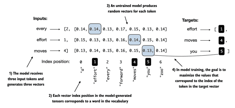
Figure 5.6 Before training, the model produces random next-token probability vectors. The goal of model training is to ensure that the probability values corresponding to the highlighted target token IDs are maximized.
The token probabilities corresponding to the target indices are as follows:
# 看看现在期望的输出的概率(probabilities)
text_idx = 0
target_probas_1 = probas[text_idx, [0, 1, 2], targets[text_idx]]
print("Text 1:", target_probas_1)

text_idx = 1
target_probas_2 = probas[text_idx, [0, 1, 2], targets[text_idx]]
print("Text 2:", target_probas_2)
# 输出
# Text 1: tensor([2.3466e-05, 2.0531e-05, 1.1733e-05])
# Text 2: tensor([4.2794e-05, 1.6248e-05, 1.1586e-05])
备注
The goal of training an LLM is to maximize these values, aiming to get them as close to a probability of 1. This way, we ensure the LLM consistently picks the target token(essentially the next word in the sentence)as the next token it generates.
Backpropagation
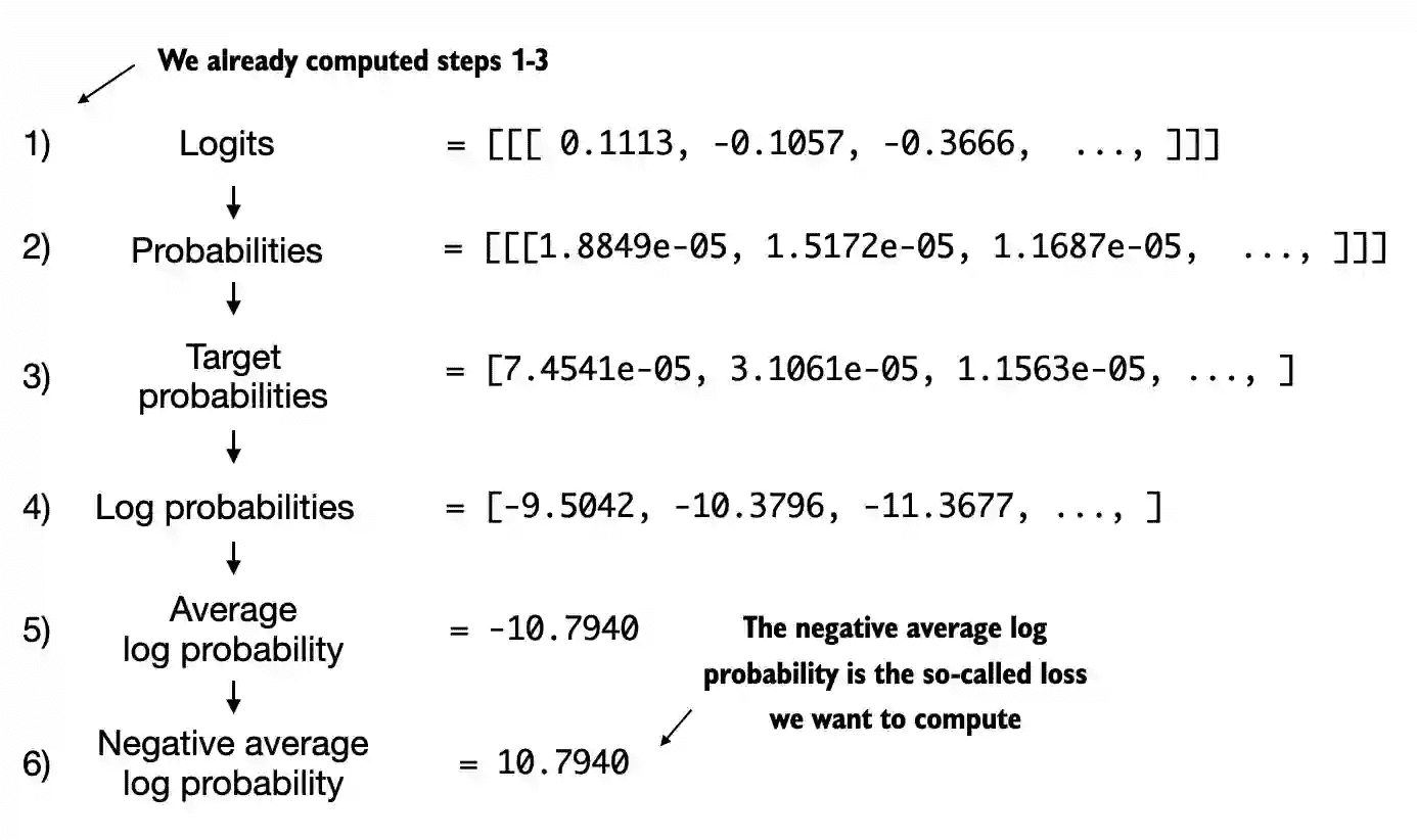
Figure 5.7 Calculating the loss involves several steps. Steps 1 to 3 calculate the token probabilities corresponding to the target tensors. These probabilities are then transformed via a logarithm and averaged in steps 4-6.
# Compute logarithm of all token probabilities
log_probas = torch.log(torch.cat((target_probas_1, target_probas_2)))
print(log_probas)
# tensor([ -9.5042, -10.3796, -11.3677, -11.4798,  -9.7764, -12.2561])

# Calculate the average probability for each token
avg_log_probas = torch.mean(log_probas)
print(avg_log_probas)
# tensor(-10.7940)

# In deep learning, the common practice is to bring the negative average log probability down to 0.
neg_avg_log_probas = avg_log_probas * -1
print(neg_avg_log_probas)
# tensor(10.7940)
备注
The term for this negative value, -10.7722 turning into 10.7722, is known as the cross entropy loss in deep learning.
Cross entropy loss
the shape of the logits and target tensors:
# Logits have shape (batch_size, num_tokens, vocab_size)
print("Logits shape:", logits.shape)
# Targets have shape (batch_size, num_tokens)
print("Targets shape:", targets.shape)
For the cross_entropy function in PyTorch, we want to flatten these tensors by combining them over the batch dimension:
logits_flat = logits.flatten(0, 1)
targets_flat = targets.flatten()
print("Flattened logits:", logits_flat.shape)
print("Flattened targets:", targets_flat.shape)
# 输出
# Flattened logits: torch.Size([6, 50257])
# Flattened targets: torch.Size([6])
PyTorch’s cross_entropy function:
loss = torch.nn.functional.cross_entropy(logits_flat, targets_flat)
print(loss)
备注
详见定义 _cross_entropy:
Perplexity
Perplexity is a measure often used alongside cross entropy loss to evaluate the performance of models in tasks like language modeling. It can provide a more interpretable way to understand the uncertainty of a model in predicting the next token in a sequence.
备注
详见定义 Perplexity 困惑度
5.1.3 Calculating the training and validation set losses
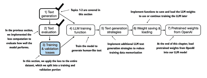
Figure 5.8 After computing the cross entropy loss in the previous section, we now apply this loss computation to the entire text dataset that we will use for model training.
The cost of pretraining LLMs
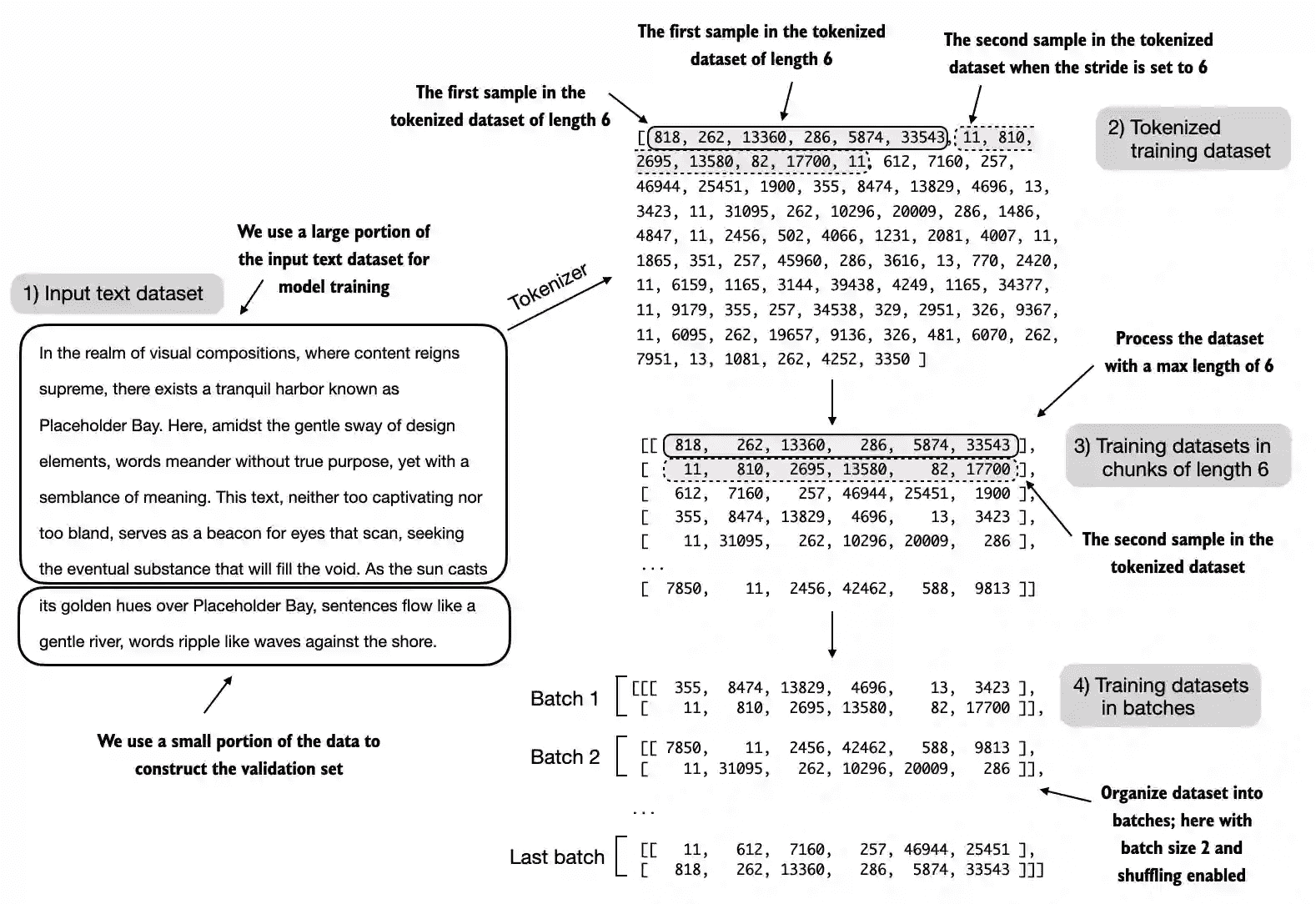
Figure 5.9 When preparing the data loaders, we split the input text into training and validation set portions. Then, we tokenize the text (only shown for the training set portion for simplicity) and divide the tokenized text into chunks of a user-specified length (here 6). Finally, we shuffle the rows and organize the chunked text into batches (here, batch size 2), which we can use for model training.
For visualization purposes, Figure 5.9 uses a max_length=6 due to spatial constraints. However, for the actual data loaders we are implementing, we set the max_length equal to the 256-token context length that the LLM supports so that the LLM sees longer texts during training.
Training with variable lengths
def calc_loss_batch(input_batch, target_batch, model, device):
    input_batch, target_batch = input_batch.to(device), target_batch.to(device)
    logits = model(input_batch)
    loss = torch.nn.functional.cross_entropy(logits.flatten(0, 1), target_batch.flatten())
    return loss


def calc_loss_loader(data_loader, model, device, num_batches=None):
    total_loss = 0.
    if len(data_loader) == 0:
        return float("nan")
    elif num_batches is None:
        num_batches = len(data_loader)
    else:
        # Reduce the number of batches to match the total number of batches in the data loader
        # if num_batches exceeds the number of batches in the data loader
        num_batches = min(num_batches, len(data_loader))
    for i, (input_batch, target_batch) in enumerate(data_loader):
        if i < num_batches:
            loss = calc_loss_batch(input_batch, target_batch, model, device)
            total_loss += loss.item()
        else:
            break
    return total_loss / num_batches


with torch.no_grad(): # Disable gradient tracking for efficiency because we are not training, yet
    train_loss = calc_loss_loader(train_loader, model, device)
    val_loss = calc_loss_loader(val_loader, model, device)

print("Training loss:", train_loss)
print("Validation loss:", val_loss)
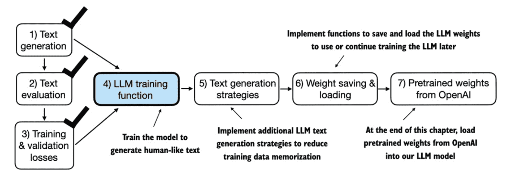
Figure 5.10 We have recapped the text generation process and implemented basic model evaluation techniques to compute the training and validation set losses. Next, we will go to the training functions and pretrain the LLM.
5.2 Training an LLM
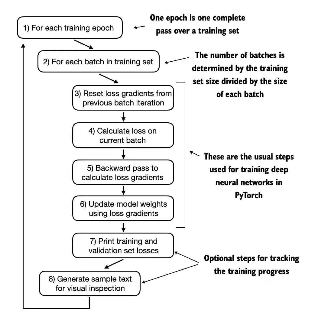
Figure 5.11 A typical training loop for training deep neural networks in PyTorch consists of several steps, iterating over the batches in the training set for several epochs. In each loop, we calculate the loss for each training set batch to determine loss gradients, which we use to update the model weights so that the training set loss is minimized.
def train_model_simple(model, train_loader, val_loader, optimizer, device, num_epochs,
                       eval_freq, eval_iter, start_context, tokenizer):
    # Initialize lists to track losses and tokens seen
    train_losses, val_losses, track_tokens_seen = [], [], []
    tokens_seen, global_step = 0, -1

    # Main training loop
    for epoch in range(num_epochs):
        model.train()  # Set model to training mode

        for input_batch, target_batch in train_loader:
            optimizer.zero_grad() # Reset loss gradients from previous batch iteration
            loss = calc_loss_batch(input_batch, target_batch, model, device)
            loss.backward() # Calculate loss gradients
            optimizer.step() # Update model weights using loss gradients
            tokens_seen += input_batch.numel()
            global_step += 1

            # Optional evaluation step
            if global_step % eval_freq == 0:
                train_loss, val_loss = evaluate_model(
                    model, train_loader, val_loader, device, eval_iter)
                train_losses.append(train_loss)
                val_losses.append(val_loss)
                track_tokens_seen.append(tokens_seen)
                print(f"Ep {epoch+1} (Step {global_step:06d}): "
                      f"Train loss {train_loss:.3f}, Val loss {val_loss:.3f}")

        # Print a sample text after each epoch
        generate_and_print_sample(
            model, tokenizer, device, start_context
        )

    return train_losses, val_losses, track_tokens_seen


def evaluate_model(model, train_loader, val_loader, device, eval_iter):
    model.eval()
    with torch.no_grad():
        train_loss = calc_loss_loader(train_loader, model, device, num_batches=eval_iter)
        val_loss = calc_loss_loader(val_loader, model, device, num_batches=eval_iter)
    model.train()
    return train_loss, val_loss


def generate_and_print_sample(model, tokenizer, device, start_context):
    model.eval()
    context_size = model.pos_emb.weight.shape[0]
    encoded = text_to_token_ids(start_context, tokenizer).to(device)
    with torch.no_grad():
        token_ids = generate_text_simple(
            model=model, idx=encoded,
            max_new_tokens=50, context_size=context_size
        )
    decoded_text = token_ids_to_text(token_ids, tokenizer)
    print(decoded_text.replace("\n", " "))  # Compact print format
    model.train()
AdamW
Adam optimizers are a popular choice for training deep neural networks.
However, in our training loop, we opt for the AdamW optimizer.
AdamW is a variant of Adam that improves the weight decay approach, which aims to minimize model complexity and prevent overfitting by penalizing(处罚) larger weights.
This adjustment allows AdamW to achieve more effective regularization and better generalization and is thus frequently used in the training of LLMs.
运行
torch.manual_seed(123)
model = GPTModel(GPT_CONFIG_124M)
model.to(device)
optimizer = torch.optim.AdamW(model.parameters(), lr=0.0004, weight_decay=0.1)

num_epochs = 10
train_losses, val_losses, tokens_seen = train_model_simple(
    model, train_loader, val_loader, optimizer, device,
    num_epochs=num_epochs, eval_freq=5, eval_iter=5,
    start_context="Every effort moves you", tokenizer=tokenizer
)
输出:
Ep 1 (Step 000000): Train loss 9.781, Val loss 9.933
Ep 1 (Step 000005): Train loss 8.111, Val loss 8.339
Every effort moves you,,,,,,,,,,,,.
Ep 2 (Step 000010): Train loss 6.661, Val loss 7.048
Ep 2 (Step 000015): Train loss 5.961, Val loss 6.616
Every effort moves you, and, and, and, and, and, and, and, and, and, and, and, and, and, and, and, and, and, and, and, and, and, and,, and, and,
... ...
Ep 9 (Step 000075): Train loss 0.717, Val loss 6.293
Ep 9 (Step 000080): Train loss 0.541, Val loss 6.393
Every effort moves you?"  "Yes--quite insensible to the irony. She wanted him vindicated--and by me!"  He laughed again, and threw back the window-curtains, I had the donkey. "There were days when I
Ep 10 (Step 000085): Train loss 0.391, Val loss 6.452
Every effort moves you know," was one of the axioms he laid down across the Sevres and silver of an exquisitely appointed luncheon-table, when, on a later day, I had again run over from Monte Carlo; and Mrs. Gis
simple plot
import matplotlib.pyplot as plt
from matplotlib.ticker import MaxNLocator


def plot_losses(epochs_seen, tokens_seen, train_losses, val_losses):
    fig, ax1 = plt.subplots(figsize=(5, 3))

    # Plot training and validation loss against epochs
    ax1.plot(epochs_seen, train_losses, label="Training loss")
    ax1.plot(epochs_seen, val_losses, linestyle="-.", label="Validation loss")
    ax1.set_xlabel("Epochs")
    ax1.set_ylabel("Loss")
    ax1.legend(loc="upper right")
    ax1.xaxis.set_major_locator(MaxNLocator(integer=True))  # only show integer labels on x-axis

    # Create a second x-axis for tokens seen
    ax2 = ax1.twiny()  # Create a second x-axis that shares the same y-axis
    ax2.plot(tokens_seen, train_losses, alpha=0)  # Invisible plot for aligning ticks
    ax2.set_xlabel("Tokens seen")

    fig.tight_layout()  # Adjust layout to make room
    plt.savefig("loss-plot.pdf")
    plt.show()

epochs_tensor = torch.linspace(0, num_epochs, len(train_losses))
plot_losses(epochs_tensor, tokens_seen, train_losses, val_losses)
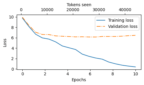
Figure 5.12 At the beginning of the training, we observe that both the training and validation set losses sharply decrease, which is a sign that the model is learning. However, the training set loss continues to decrease past the second epoch, whereas the validation loss stagnates. This is a sign that the model is still learning, but it’s overfitting to the training set past epoch 2.
小结
Looking at the results above, we can see that the model starts out generating incomprehensible strings of words, whereas towards the end, it’s able to produce grammatically more or less correct sentences
However, based on the training and validation set losses, we can see that the model starts overfitting(最终训练集损失是0.541,而验证集损失是6.393)
If we were to check a few passages it writes towards the end, we would find that they are contained in the training set verbatim(逐字翻译) – it simply memorizes the training data
Later, we will cover decoding strategies that can mitigate this memorization by a certain degree
Note that the overfitting here occurs because we have a very, very small training set, and we iterate over it so many times
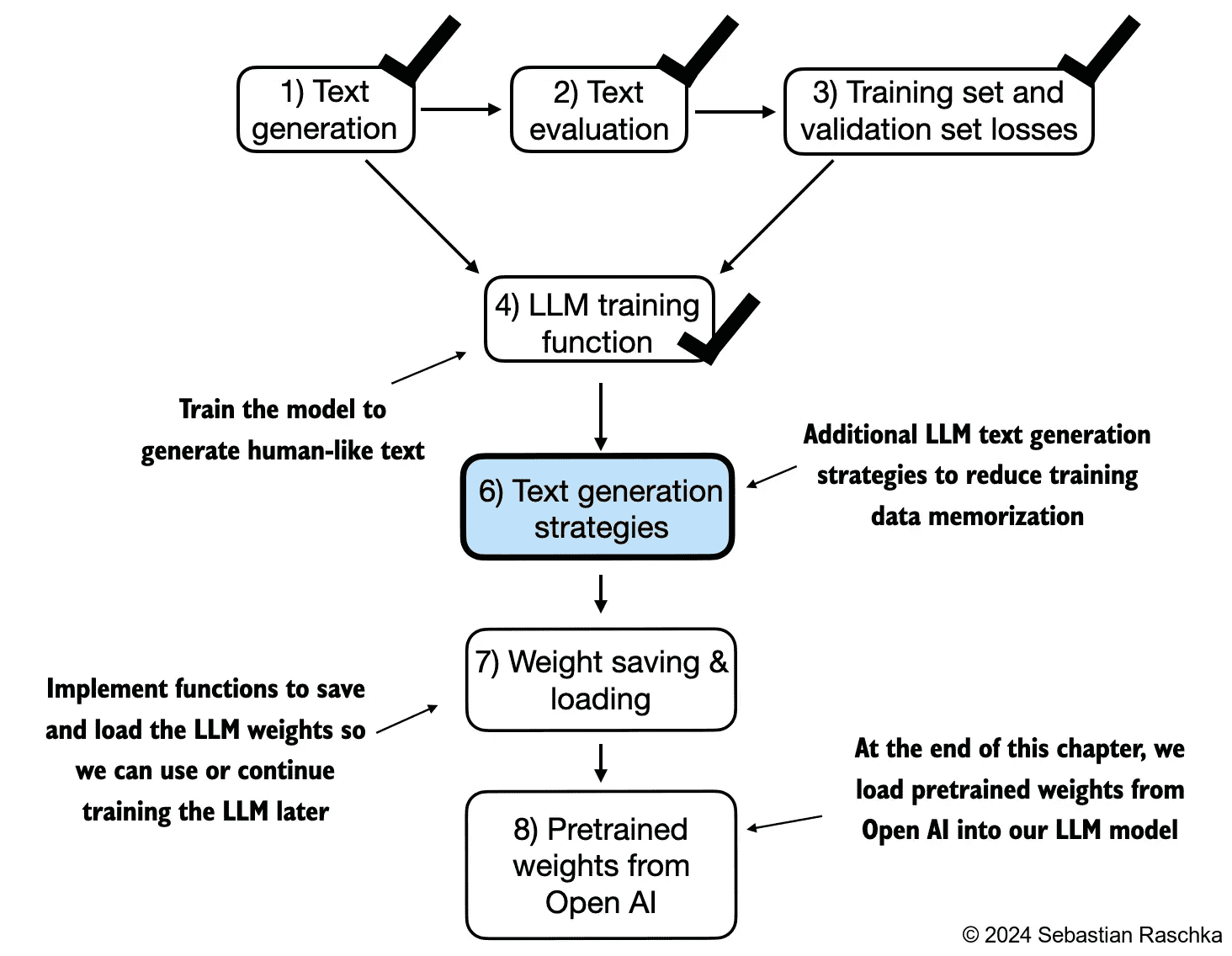
Figure 5.13 Our model can generate coherent text after implementing the training function. However, it often memorizes passages from the training set verbatim. The following section covers strategies to generate more diverse output texts.
5.3 Decoding strategies to control randomness
本节将重新实现
generate_text_simple() in chapter 4.7但 we will cover two techniques, temperature scaling, and top-k sampling, to improve this function.之前实现的版本使用的贪心解码(greedy decoding),每一次请求的返回结果都是选择概率最高的那个,导致每一次请求的结果都是相同的,这样对生成式的任务而言,效果单一。
5.3.1 Temperature scaling
This section introduces
temperature scaling, a technique that adds a probabilistic selection process to the next-token generation task.Previously, inside the
generate_text_simplefunction, we always sampled the token with the highest probability as the next token usingtorch.argmax, also known asgreedy decoding. To generate text with more variety, we can replace the argmax with a function thatsamples from a probability distribution(here, the probability scores the LLM generates for each vocabulary entry at each token generation step).
small vocabulary for illustration purposes:
vocab = {
    "closer": 0,
    "every": 1,
    "effort": 2,
    "forward": 3,
    "inches": 4,
    "moves": 5,
    "pizza": 6,
    "toward": 7,
    "you": 8,
}
inverse_vocab = {v: k for k, v in vocab.items()}
上节讲的 greedy decoding
next_token_logits = torch.tensor(
    [4.51, 0.89, -1.90, 6.75, 1.63, -1.62, -1.89, 6.28, 1.79]
)
probas = torch.softmax(next_token_logits, dim=0)
next_token_id = torch.argmax(probas).item()
print(inverse_vocab[next_token_id])
# "forward"
# 讲解:
#   通过对 next_token_logits 分析知道
#   最大概率是 6.75, 对应的softmax的最大值
#   所以next token的index是3,得到最终结果: forward
对应的 probabilistic sampling process
# replace the argmax with the multinomial function in PyTorch
torch.manual_seed(123)
next_token_id = torch.multinomial(probas, num_samples=1).item()
print(inverse_vocab[next_token_id])
# 说明: 不管概率高低,都有被选中的可能
temperature scaling 的作用:
# Temperatures greater than 1 result in more uniformly distributed token probabilities
# Temperatures smaller than 1 will result in more confident (sharper or more peaky) distributions.
def softmax_with_temperature(logits, temperature):
    scaled_logits = logits / temperature
    return torch.softmax(scaled_logits, dim=0)
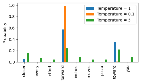
Figure 5.14 A temperature of 1 represents the unscaled probability scores for each token in the vocabulary. Decreasing the temperature to 0.1 sharpens the distribution, so the most likely token (here “forward”) will have an even higher probability score. Vice versa, increasing the temperature to 5 makes the distribution more uniform.
5.3.2 Top-k sampling
上节的方法allows for exploring less likely but potentially more interesting and creative paths in the generation process. However, One downside of this approach is that it sometimes leads to grammatically incorrect or completely nonsensicaloutputs(就是超低概率被命中,正常来说这种nexttoken是不太合适的,也就是无意义的语句生成)
备注
In top-k sampling, we can restrict the sampled tokens to the top-k most likely tokens and exclude all other tokens from the selection process by masking their probability scores
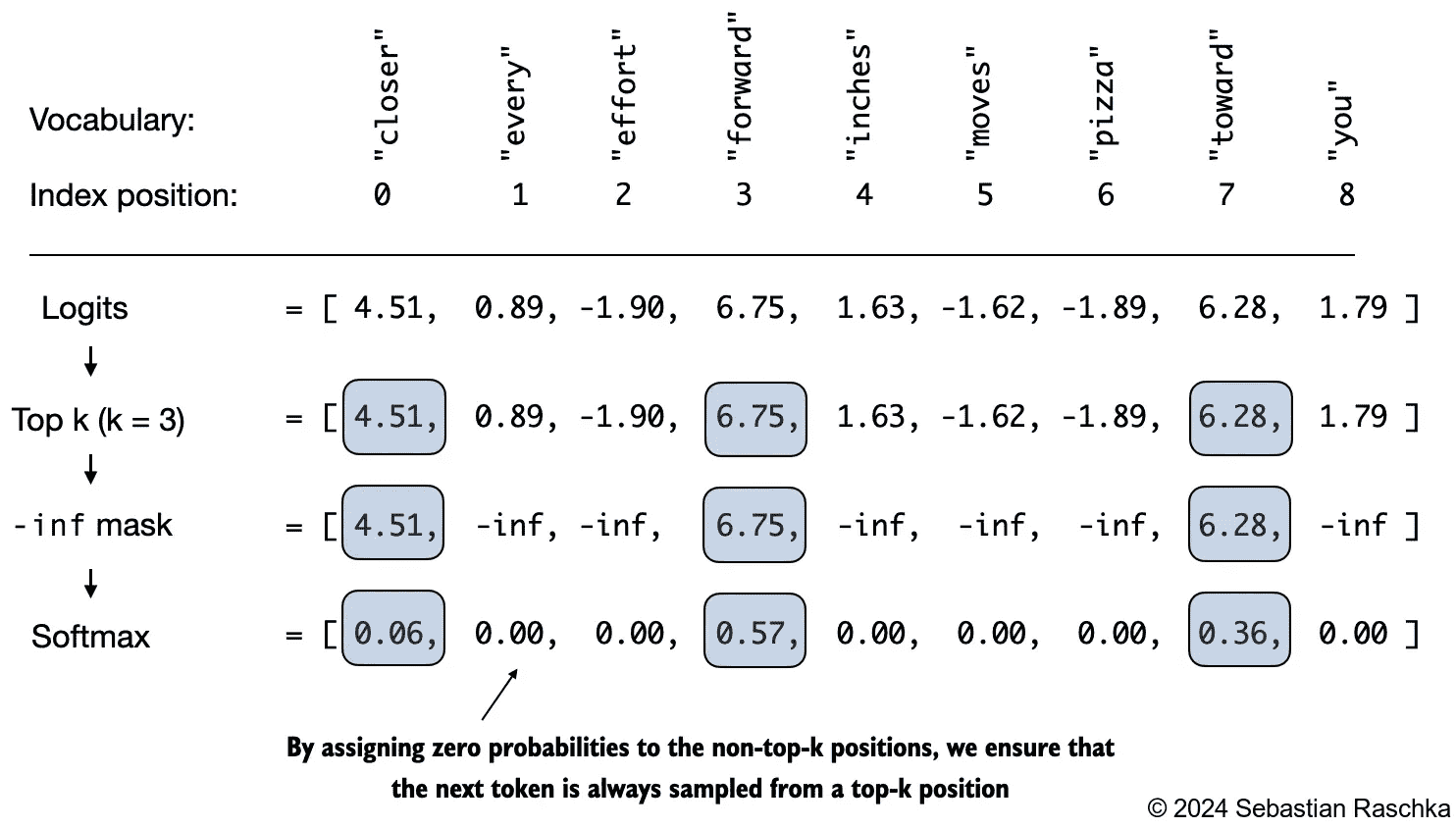
Figure 5.15 Using top-k sampling with k=3, we focus on the 3 tokens associated with the highest logits and mask out all other tokens with negative infinity (-inf) before applying the softmax function. This results in a probability distribution with a probability value 0 assigned to all non- top-k tokens.
top_k = 3
top_logits, top_pos = torch.topk(next_token_logits, top_k)
new_logits = torch.where(
    condition=next_token_logits < top_logits[-1],
    input=torch.tensor(float("-inf")),
    other=next_token_logits
)
topk_probas = torch.softmax(new_logits, dim=0)

# 更高效实现
> new_logits = torch.full_like( # create tensor containing -inf values
>    next_token_logits, -torch.inf
>)
> new_logits[top_pos] = next_token_logits[top_pos] # copy top k values into the -inf tensor
> topk_probas = torch.softmax(new_logits, dim=0)
top_p(也称为核采样或nucleus sampling): 算法会首先将所有词按其概率排序,然后累积这些概率直到总和首次达到或超过 p 值。随后,只从这个累积概率达到了 p 的词集中随机抽样选择下一个词,而忽略其余概率较低的词。例如,如果设置 top_p=0.9,则会选择最小的词集,使得它们的累积概率至少为 90%,并从这个集合中随机抽取下一个词。
备注
当同时设置 top_k 和 top_p 时:先执行 top_k:首先从模型预测的概率分布中选择概率最高的前 k 个词。然后应用 top_p:在通过 top_k 筛选后的词汇集合中,进一步筛选出累积概率达到或超过 p 的最小词集。这意味着即使某个词在 top_k 范围内,如果它的累积概率超过了设定的 p 值,它也可能不会被考虑。
5.3.3 Modifying the text generation function
本节把前面两节的 temperature scale 和 top-k sampling 合并到generator函数中
def generate(model, idx, max_new_tokens, context_size, temperature=0.0, top_k=None, eos_id=None):
    # For-loop is the same as before: Get logits, and only focus on last time step
    for _ in range(max_new_tokens):
        idx_cond = idx[:, -context_size:]
        with torch.no_grad():
            logits = model(idx_cond)
        logits = logits[:, -1, :]

        # New: Filter logits with top_k sampling
        if top_k is not None:
            # Keep only top_k values
            top_logits, _ = torch.topk(logits, top_k)
            min_val = top_logits[:, -1]
            logits = torch.where(logits < min_val, torch.tensor(float("-inf")).to(logits.device), logits)

        # New: Apply temperature scaling
        if temperature > 0.0:
            logits = logits / temperature

            # Apply softmax to get probabilities
            probs = torch.softmax(logits, dim=-1)  # (batch_size, context_len)

            # Sample from the distribution
            idx_next = torch.multinomial(probs, num_samples=1)  # (batch_size, 1)

        # Otherwise same as before: get idx of the vocab entry with the highest logits value
        else:
            idx_next = torch.argmax(logits, dim=-1, keepdim=True)  # (batch_size, 1)

        if idx_next == eos_id:  # Stop generating early if end-of-sequence token is encountered and eos_id is specified
            break

        # Same as before: append sampled index to the running sequence
        idx = torch.cat((idx, idx_next), dim=1)  # (batch_size, num_tokens+1)
5.4 Loading and saving model weights in PyTorch
It’s common to train LLMs with adaptive optimizers like Adam or AdamW instead of regular SGD
These adaptive optimizers store additional parameters for each model weight, so it makes sense to save them as well in case we plan to continue the pretraining later:
torch.save({
    "model_state_dict": model.state_dict(),
    "optimizer_state_dict": optimizer.state_dict(),
    },
    "model_and_optimizer.pth"
)
loading:
checkpoint = torch.load("model_and_optimizer.pth", weights_only=True)

model = GPTModel(GPT_CONFIG_124M)
model.load_state_dict(checkpoint["model_state_dict"])

optimizer = torch.optim.AdamW(model.parameters(), lr=0.0005, weight_decay=0.1)
optimizer.load_state_dict(checkpoint["optimizer_state_dict"])
model.train();
5.5 Loading pretrained weights from OpenAI
本节主要讲了,如何从gpt2中加载权重
因为gpt2和我们这儿定义的数据结构名称不相同,所以需要专门进行定制加载
5.6 Summary
When LLMs generate text, they output one token at a time.
By default, the next token is generated by converting the model outputs into probability scores and selecting the token from the vocabulary that corresponds to the highest probability score, which is known as “greedy decoding.”
Using probabilistic sampling and temperature scaling, we can influence the diversity and coherence of the generated text.
Training and validation set losses can be used to gauge(测量) the quality of text generated by LLM during training.
Pretraining an LLM involves changing its weights to minimize the training loss.
The training loop for LLMs itself is a standard procedure in deep learning, using a conventional
cross entropy lossandAdamW optimizer. Pretraining an LLM on a large text corpus is time- and resource- intensive so we can load openly available weights from OpenAI as an alternative to pretraining the model on a large dataset ourselves.
6 Fine-tuning for classification
Introducing different LLM fine-tuning approaches
Preparing a dataset for text classification
Modifying a pretrained LLM for fine-tuning
Fine-tuning an LLM to identify spam messages
Evaluating the accuracy of a fine-tuned LLM classifier
Using a fine-tuned LLM to classify new data
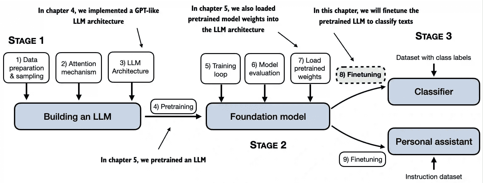
Figure 6.1 The three main stages of coding an LLM. This chapter focus on stage 3 (step 8): fine-tuning a pretrained LLM as a classifier.
6.1 Different categories of fine-tuning
The most common ways to fine-tune language models are
instruction fine-tuningandclassification fine-tuning.Instruction fine-tuninginvolves training a language model on a set of tasks using specific instructions to improve its ability to understand and execute tasks described in natural language prompts
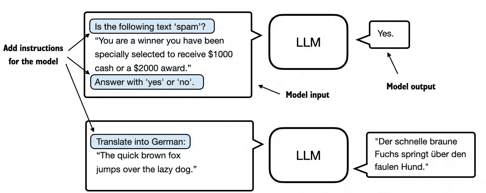
Figure 6.2 Two different instruction fine-tuning scenarios. At the top, the model is tasked with determining whether a given text is spam. At the bottom, the model is given an instruction on how to translate an English sentence into German.
备注
Instruction-finetuning, depicted below, is the topic of the next chapter. 本节主要讲 text classification.
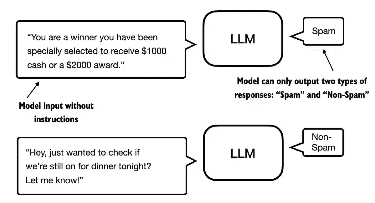
Figure 6.3 A text classification scenario using an LLM. A model fine-tuned for spam classification does not require further instruction alongside the input. In contrast to an instruction fine-tuned model, it can only respond with “spam” or “not spam.”
Classification finetuning, the topic of this chapter, is a procedure you may already be familiar with if you have a background in machine learning – it’s similar to training a convolutional network to classify handwritten digits, for example
In classification finetuning, we have a specific number of class labels (for example, “spam” and “not spam”) that the model can output
A classification finetuned model can only predict classes it has seen during training (for example, “spam” or “not spam”), whereas an instruction-finetuned model can usually perform many tasks
备注
We can think of a classification-finetuned model as a very specialized model; in practice, it is much easier to create a specialized model than a generalist model that performs well on many different tasks
CHOOSING THE RIGHT APPROACH
Instruction fine-tuning improves a model’s ability to understand and generate responses based on specific user instructions. Instruction fine-tuning is best suited for models that need to handle a variety of tasks based on complex user instructions, improving flexibility and interaction quality. Classification fine-tuning is ideal for projects requiring precise categorization of data into predefined classes, such as sentiment analysis or spam detection.
While instruction fine-tuning is more versatile, it demands larger datasets and greater computational resources to develop models proficient in various tasks. In contrast, classification fine-tuning requires less data and compute power, but its use is confined to the specific classes on which the model has been trained.
6.2 Preparing the dataset
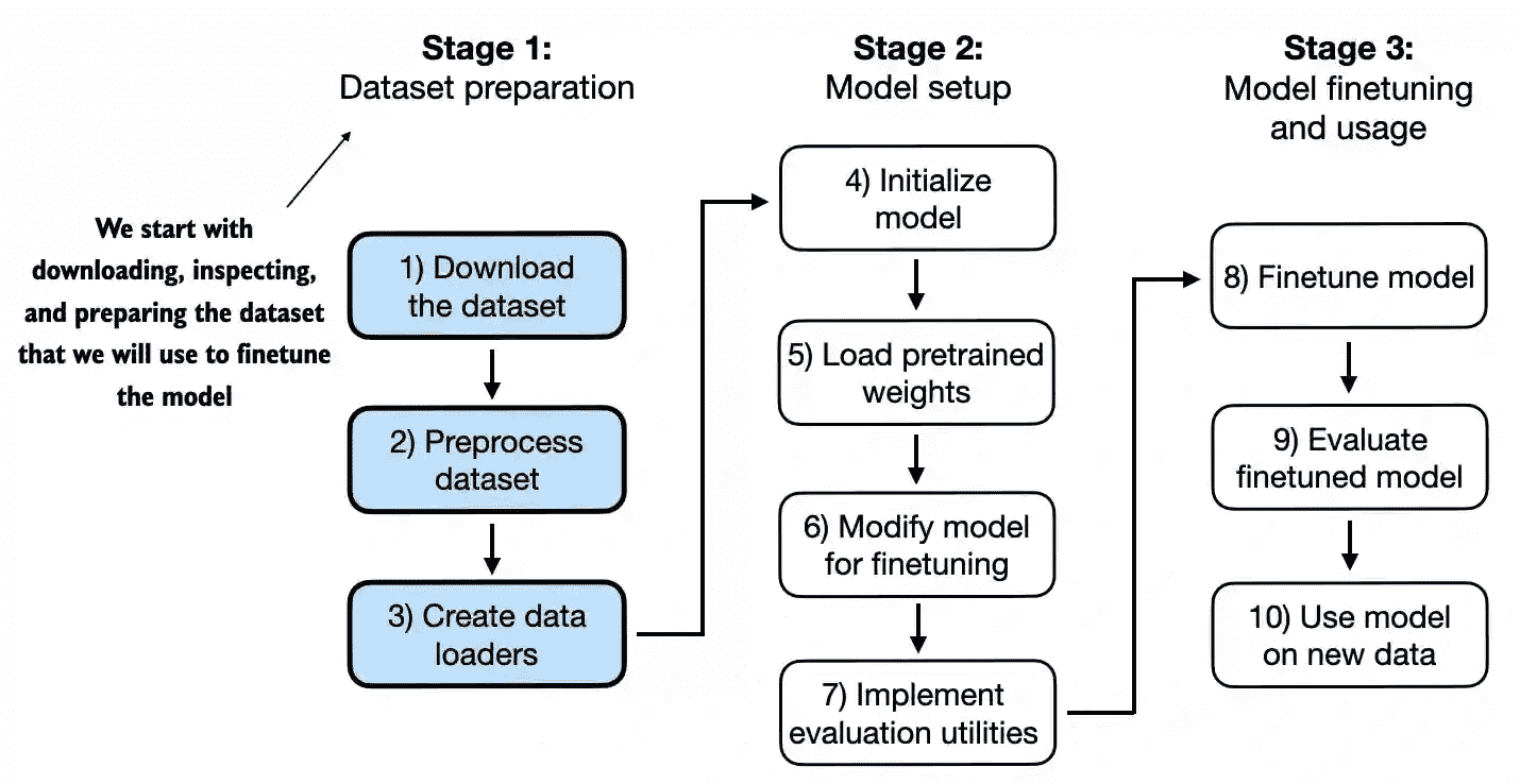
Figure 6.4 The three-stage process for classification fine- tuning an LLM. Stage 1 involves dataset preparation. Stage 2 focuses on model setup. Stage 3 covers fine-tuning and evaluating the model.
url = "https://archive.ics.uci.edu/static/public/228/sms+spam+collection.zip"
=>
提取出3个数据集:
train_df.to_csv("train.csv", index=None)
validation_df.to_csv("validation.csv", index=None)
test_df.to_csv("test.csv", index=None)
6.3 Creating data loaders
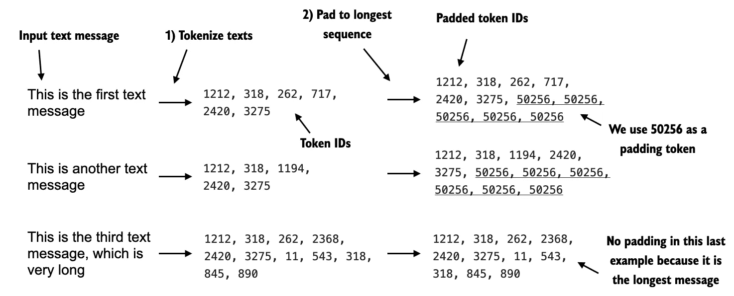
we use <|endoftext|> as a padding token
import torch
from torch.utils.data import Dataset

class SpamDataset(Dataset):
    def __init__(self, csv_file, tokenizer, max_length=None, pad_token_id=50256):
        self.data = pd.read_csv(csv_file)

        # Pre-tokenize texts
        self.encoded_texts = [
            tokenizer.encode(text) for text in self.data["Text"]
        ]

        if max_length is None:
            self.max_length = self._longest_encoded_length()
        else:
            self.max_length = max_length
            # Truncate sequences if they are longer than max_length
            self.encoded_texts = [
                encoded_text[:self.max_length]
                for encoded_text in self.encoded_texts
            ]

        # Pad sequences to the longest sequence
        self.encoded_texts = [
            encoded_text + [pad_token_id] * (self.max_length - len(encoded_text))
            for encoded_text in self.encoded_texts
        ]

    def __getitem__(self, index):
        encoded = self.encoded_texts[index]
        label = self.data.iloc[index]["Label"]
        return (
            torch.tensor(encoded, dtype=torch.long),
            torch.tensor(label, dtype=torch.long)
        )

    def __len__(self):
        return len(self.data)

    def _longest_encoded_length(self):
        max_length = 0
        for encoded_text in self.encoded_texts:
            encoded_length = len(encoded_text)
            if encoded_length > max_length:
                max_length = encoded_length
        return max_length
使用:
train_dataset = SpamDataset(
    csv_file="train.csv",
    max_length=None,
    tokenizer=tokenizer
)
验证集和测试集可以设定max_length(也可以和训练集一样设置max_length=None):
val_dataset = SpamDataset(
    csv_file="validation.csv",
    max_length=train_dataset.max_length,
    tokenizer=tokenizer
)
test_dataset = SpamDataset(
    csv_file="test.csv",
    max_length=train_dataset.max_length,
    tokenizer=tokenizer
)
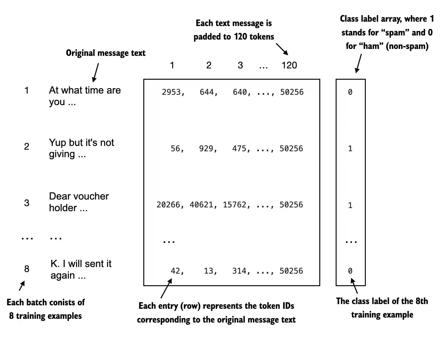
Figure 6.7 A single training batch consisting of eight text messages represented as token IDs. Each text message consists of 120 token IDs. A class label array stores the eight class labels corresponding to the text messages, which can be either 0 (“not spam”) or 1 (“spam”).
data loaders(以训练集示例):
from torch.utils.data import DataLoader

num_workers = 0
batch_size = 8
train_loader = DataLoader(
    dataset=train_dataset,
    batch_size=batch_size,
    shuffle=True,
    num_workers=num_workers,
    drop_last=True,
)
6.4 Initializing a model with pretrained weights
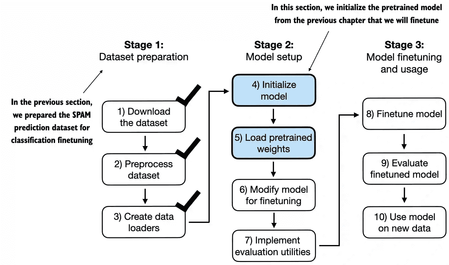
Figure 6.8 The three-stage process for classification fine- tuning the LLM. Having completed stage 1, preparing the dataset, we now must initialize the LLM, which we will then fine-tune to classify spam messages.
用前面章节实现模型的初始化和加载gpt2的权重:
... ...
model = GPTModel(BASE_CONFIG)
load_weights_into_gpt(model, params)
model.eval();
6.5 Adding a classification head
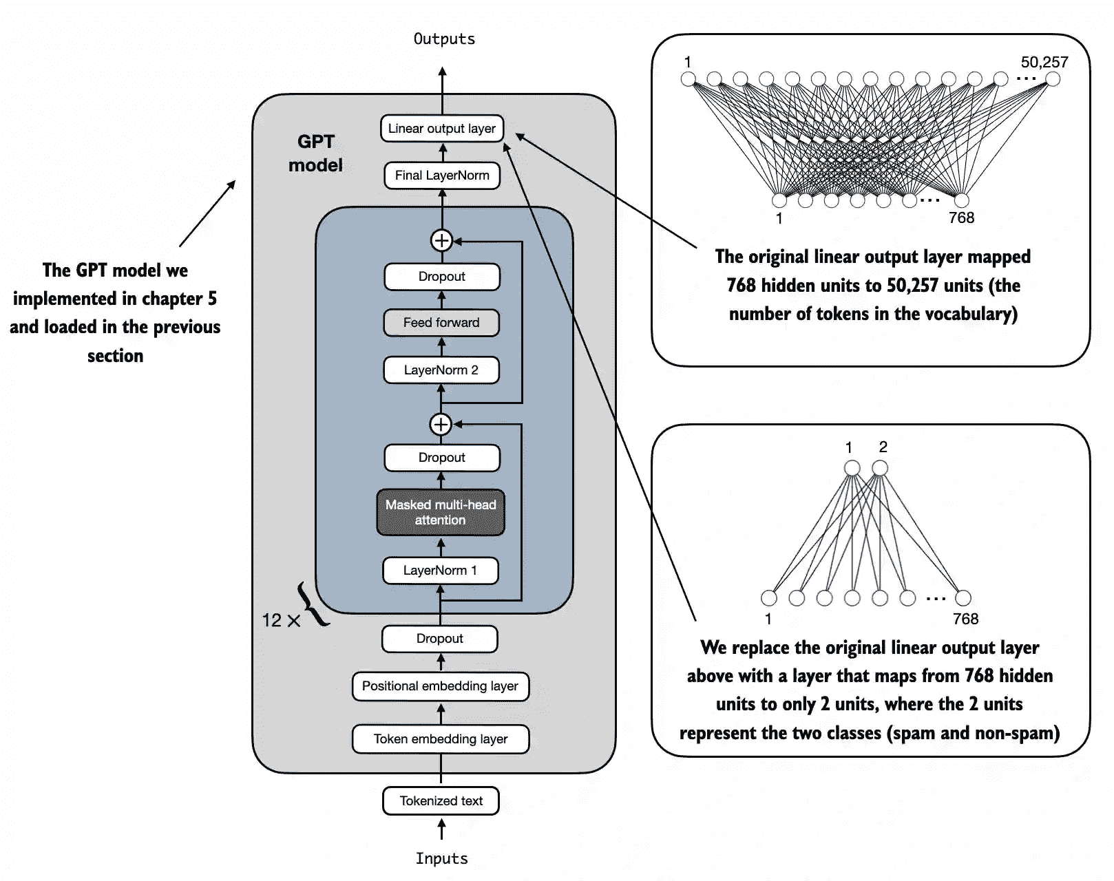
Figure 6.9 Adapting a GPT model for spam classification by altering its architecture. Initially, the model’s linear output layer mapped 768 hidden units to a vocabulary of 50,257 tokens. To detect spam, we replace this layer with a new output layer that maps the same 768 hidden units to just two classes, representing “spam” and “not spam.”
OUTPUT LAYER NODES
print the model architecture via print(model)
GPTModel(
  (tok_emb): Embedding(50257, 768)
  (pos_emb): Embedding(1024, 768)
  (drop_emb): Dropout(p=0.0, inplace=False)
  (trf_blocks): Sequential(
    (0): TransformerBlock(
      (att): MultiHeadAttention(
        (W_query): Linear(in_features=768, out_features=768, bias=True)
        (W_key): Linear(in_features=768, out_features=768, bias=True)
        (W_value): Linear(in_features=768, out_features=768, bias=True)
        (out_proj): Linear(in_features=768, out_features=768, bias=True)
        (dropout): Dropout(p=0.0, inplace=False)
      )
      (ff): FeedForward(
        (layers): Sequential(
          (0): Linear(in_features=768, out_features=3072, bias=True)
          (1): GELU()
          (2): Linear(in_features=3072, out_features=768, bias=True)
        )
      )
      (norm1): LayerNorm()
      (norm2): LayerNorm()
      (drop_resid): Dropout(p=0.0, inplace=False)
    )
   ... ... # 省略11个
  )
  (final_norm): LayerNorm()
  (out_head): Linear(in_features=768, out_features=50257, bias=False)
)
FINE-TUNING SELECTED LAYERS VS. ALL LAYERS
The goal is to replace and finetune the output layer
To achieve this, we first freeze the model, meaning that we make all layers non-trainable:
for param in model.parameters():
    param.requires_grad = False
Then, we replace the output layer (model.out_head):
# finetune the model for binary classification (predicting 2 classes, "spam" and "not spam")
torch.manual_seed(123)
num_classes = 2
model.out_head = torch.nn.Linear(in_features=BASE_CONFIG["emb_dim"], out_features=num_classes)
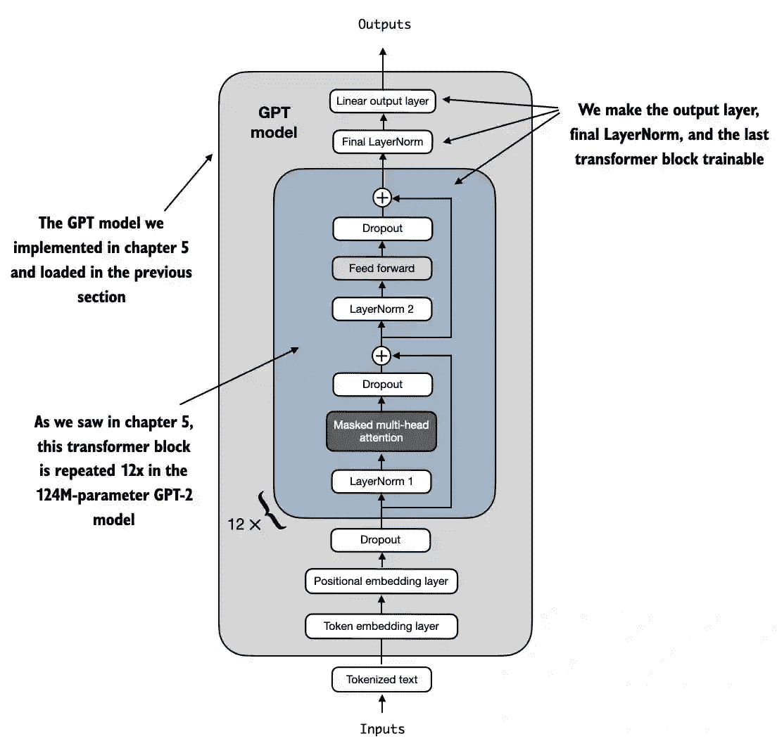
Figure 6.10 The GPT model includes 12 repeated transformer blocks. Alongside the output layer, we set the final LayerNorm and the last transformer block as trainable. The remaining 11 transformer blocks and the embedding layers are kept nontrainable.
Technically, it’s sufficient to only train the output layer
However, as I found in Finetuning Large Language Models , experiments show that finetuning additional layers can noticeably improve the performance
So, we are also making the last transformer block and the final LayerNorm module connecting the last transformer block to the output layer trainable
for param in model.trf_blocks[-1].parameters():
    param.requires_grad = True

for param in model.final_norm.parameters():
    param.requires_grad = True

Figure 6.11 The GPT model with a four-token example input and output. The output tensor consists of two columns due to the modified output layer. We are only interested in the last row corresponding to the last token when fine-tuning the model for spam classification.
In chapter 3, we discussed the attention mechanism, which connects each input token to each other input token
In chapter 3, we then also introduced the causal attention mask that is used in GPT-like models; this causal mask lets a current token only attend to the current and previous token positions
Based on this causal attention mechanism, the 4th (last) token contains the most information among all tokens because it’s the only token that includes information about all other tokens
Hence, we are particularly interested in this last token, which we will finetune for the spam classification task
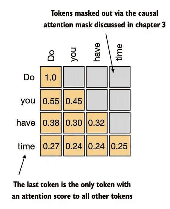
Figure 6.12 The causal attention mechanism, where the attention scores between input tokens are displayed in a matrix format. The empty cells indicate masked positions due to the causal attention mask, preventing tokens from attending to future tokens. The values in the cells represent attention scores; the last token, time , is the only one that computes attention scores for all preceding tokens.
6.6 Calculating the classification loss and accuracy
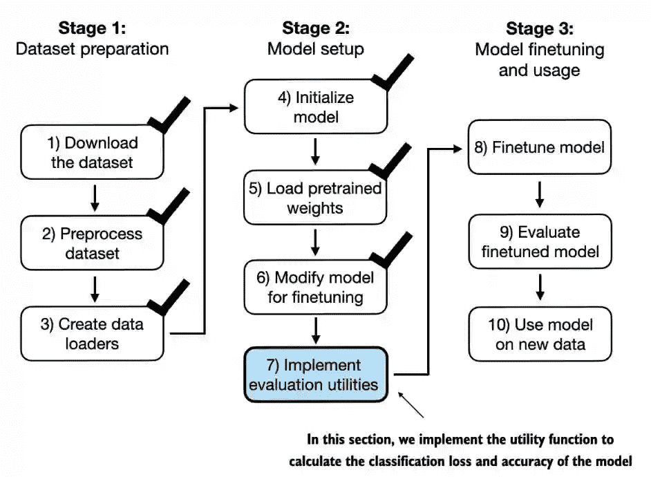
Figure 6.13 The three-stage process for classification fine- tuning the LLM. We’ve completed the first six steps. We are now ready to undertake the last step of stage 2: implementing the functions to evaluate the model’s performance to classify spam messages before, during, and after the fine-tuning.
We previously computed the token ID of the next token generated by the LLM by converting the 50,257 outputs into probabilities via the softmax function and then returning the position of the highest probability via the argmax function.
We take the same approach here to calculate whether the model outputs a “spam” or “not spam” prediction for a given input, as shown in figure 6.14.
The only difference is that we work with 2-dimensional instead of 50,257-dimensional outputs.
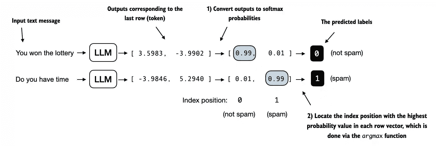
Figure 6.14 The model outputs corresponding to the last token are converted into probability scores for each input text. The class labels are obtained by looking up the index position of the highest probability score. The model predicts the spam labels incorrectly because it has not yet been trained.
Note that the softmax function is optional here:
logits = outputs[:, -1, :]
label = torch.argmax(logits)
print("Class label:", label.item())
Compute the classification accuracy, which measures the percentage of correct predictions across a dataset.
def calc_accuracy_loader(data_loader, model, device, num_batches=None):
    model.eval()
    correct_predictions, num_examples = 0, 0

    if num_batches is None:
        num_batches = len(data_loader)
    else:
        num_batches = min(num_batches, len(data_loader))
    for i, (input_batch, target_batch) in enumerate(data_loader):
        if i < num_batches:
            input_batch, target_batch = input_batch.to(device), target_batch.to(device)

            with torch.no_grad():
                logits = model(input_batch)[:, -1, :]  # Logits of last output token
            predicted_labels = torch.argmax(logits, dim=-1)

            num_examples += predicted_labels.shape[0]
            correct_predictions += (predicted_labels == target_batch).sum().item()
        else:
            break
    return correct_predictions / num_examples
use the function to determine the classification accuracies across various datasets:
train_accuracy = calc_accuracy_loader(train_loader, model, device, num_batches=10)
print(f"Training accuracy: {train_accuracy*100:.2f}%")

...  # 验证和测试集相同做法
Because classification accuracy is not a differentiable function, we use cross-entropy loss as a proxy to maximize accuracy.
Accordingly, the
calc_loss_batchfunction remains the same, with one adjustment: we focus on optimizing only the last token,model(input_batch)[:, -1, :], rather than all tokens,model(input_batch)
def calc_loss_batch(input_batch, target_batch, model, device):
    input_batch, target_batch = input_batch.to(device), target_batch.to(device)
    logits = model(input_batch)[:, -1, :]  # Logits of last output token
    loss = torch.nn.functional.cross_entropy(logits, target_batch)
    return loss
The
calc_loss_loaderis exactly the same as in chapter 5Using the
calc_closs_loader, we compute the initial training, validation, and test set losses before we start training- with torch.no_grad(): # Disable gradient tracking for efficiency because we are not training, yet
train_loss = calc_loss_loader(train_loader, model, device, num_batches=5) val_loss = calc_loss_loader(val_loader, model, device, num_batches=5) test_loss = calc_loss_loader(test_loader, model, device, num_batches=5)
print(f”Training loss: {train_loss:.3f}”) print(f”Validation loss: {val_loss:.3f}”) print(f”Test loss: {test_loss:.3f}”)
6.7 Finetuning the model on supervised data
We must define and use the training function to fine-tune the pretrained LLM and improve its spam classification accuracy.
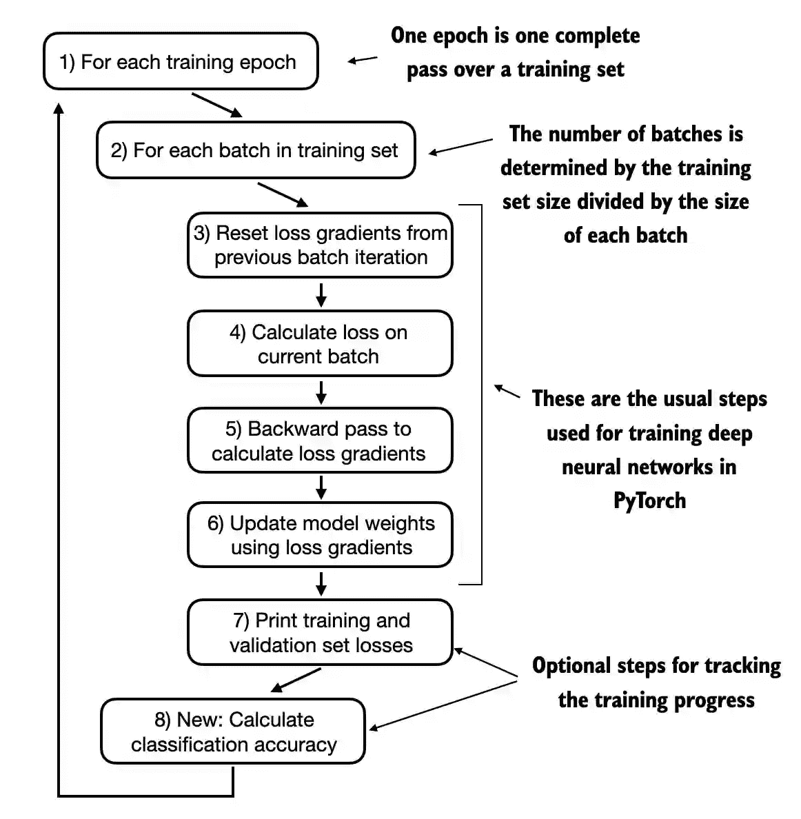
Figure 6.15 A typical training loop for training deep neural networks in PyTorch consists of several steps, iterating over the batches in the training set for several epochs. In each loop, we calculate the loss for each training set batch to determine loss gradients, which we use to update the model weights to minimize the training set loss.
Overall the same as
train_model_simplein chapter 5
def train_classifier_simple(model, train_loader, val_loader, optimizer, device, num_epochs,
                            eval_freq, eval_iter):
    # Initialize lists to track losses and examples seen
    train_losses, val_losses, train_accs, val_accs = [], [], [], []
    examples_seen, global_step = 0, -1

    # Main training loop
    for epoch in range(num_epochs):
        model.train()  # Set model to training mode

        for input_batch, target_batch in train_loader:
            optimizer.zero_grad() # Reset loss gradients from previous batch iteration
            loss = calc_loss_batch(input_batch, target_batch, model, device)
            loss.backward() # Calculate loss gradients
            optimizer.step() # Update model weights using loss gradients
            examples_seen += input_batch.shape[0] # New: track examples instead of tokens
            global_step += 1

            # Optional evaluation step
            if global_step % eval_freq == 0:
                train_loss, val_loss = evaluate_model(
                    model, train_loader, val_loader, device, eval_iter)
                train_losses.append(train_loss)
                val_losses.append(val_loss)
                print(f"Ep {epoch+1} (Step {global_step:06d}): "
                      f"Train loss {train_loss:.3f}, Val loss {val_loss:.3f}")

        # Calculate accuracy after each epoch
        train_accuracy = calc_accuracy_loader(train_loader, model, device, num_batches=eval_iter)
        val_accuracy = calc_accuracy_loader(val_loader, model, device, num_batches=eval_iter)
        print(f"Training accuracy: {train_accuracy*100:.2f}% | ", end="")
        print(f"Validation accuracy: {val_accuracy*100:.2f}%")
        train_accs.append(train_accuracy)
        val_accs.append(val_accuracy)

    return train_losses, val_losses, train_accs, val_accs, examples_seen
The
evaluate_modelfunction used in thetrain_classifier_simpleis the same as the one we used in chapter 5:# Same as chapter 5 def evaluate_model(model, train_loader, val_loader, device, eval_iter): model.eval() with torch.no_grad(): train_loss = calc_loss_loader(train_loader, model, device, num_batches=eval_iter) val_loss = calc_loss_loader(val_loader, model, device, num_batches=eval_iter) model.train() return train_loss, val_loss
The training takes about 5 minutes on a M3 MacBook Air laptop computer and less than half a minute on a V100 or A100 GPU
optimizer = torch.optim.AdamW(model.parameters(), lr=5e-5, weight_decay=0.1)

num_epochs = 5
train_losses, val_losses, train_accs, val_accs, examples_seen = train_classifier_simple(
    model, train_loader, val_loader, optimizer, device,
    num_epochs=num_epochs, eval_freq=50, eval_iter=5,
)
The resulting accuracy values are:
Training accuracy: 97.21%
Validation accuracy: 97.32%
Test accuracy: 95.67%
CHOOSING THE NUMBER OF EPOCHS
The number of epochs depends on the dataset and the task’s difficulty, and there is no universal solution or recommendation, although an epoch number of five is usually a good starting point.
If the model overfits after the first few epochs as a loss plot, you may need to reduce the number of epochs.
If the trendline suggests that the validation loss could improve with further training, you should increase the number of epochs.
6.8 Using the LLM as a spam classifier
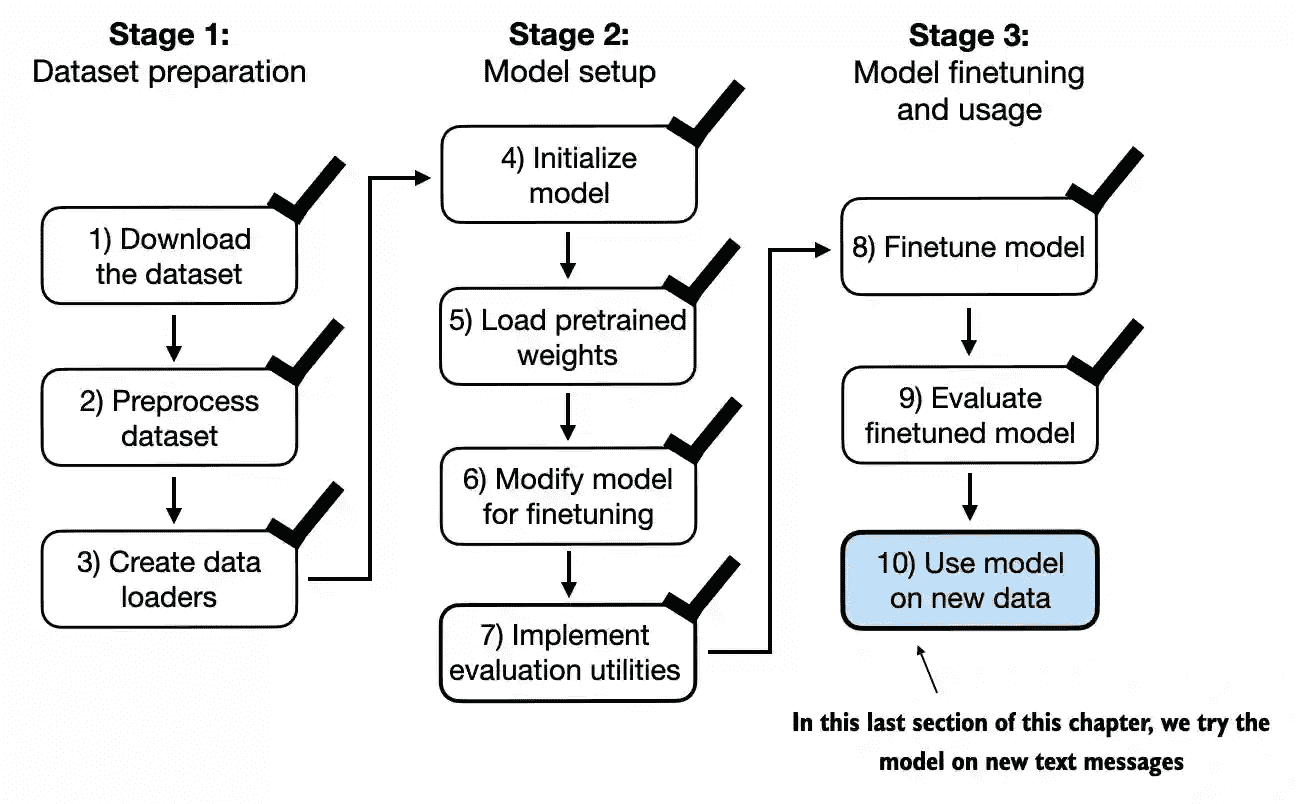
Figure 6.18 The three-stage process for classification fine- tuning our LLM. Step 10 is the final step of stage 3—using the fine-tuned model to classify new spam messages.
Summary
There are different strategies for fine-tuning LLMs, including classification fine-tuning and instruction fine-tuning.
Classification fine-tuning involves replacing the output layer of an LLM via a small classification layer.
In the case of classifying text messages as “spam” or “not spam,” the new classification layer consists of only two output nodes.
Previously, we used the number of output nodes equal to the number of unique tokens in the vocabulary (i.e., 50,256).
Instead of predicting the next token in the text as in pretraining, classification fine-tuning trains the model to output a correct class label—for example, “spam” or “not spam.”
The model input for fine-tuning is text converted into token IDs, similar to pretraining.
Before fine-tuning an LLM, we load the pretrained model as a base model.
Evaluating a classification model involves calculating the classification accuracy (the fraction or percentage of correct predictions).
Fine-tuning a classification model uses the same cross entropy loss function as when pretraining the LLM.
7 Fine-tuning to follow instructions
This chapter covers
The instruction fine-tuning process of LLMs
Preparing a dataset for supervised instruction fine-tuning Organizing instruction data in training batches
Loading a pretrained LLM and fine-tuning it to follow human instructions
Extracting LLM-generated instruction responses for evaluation
Evaluating an instruction-fine-tuned LLM
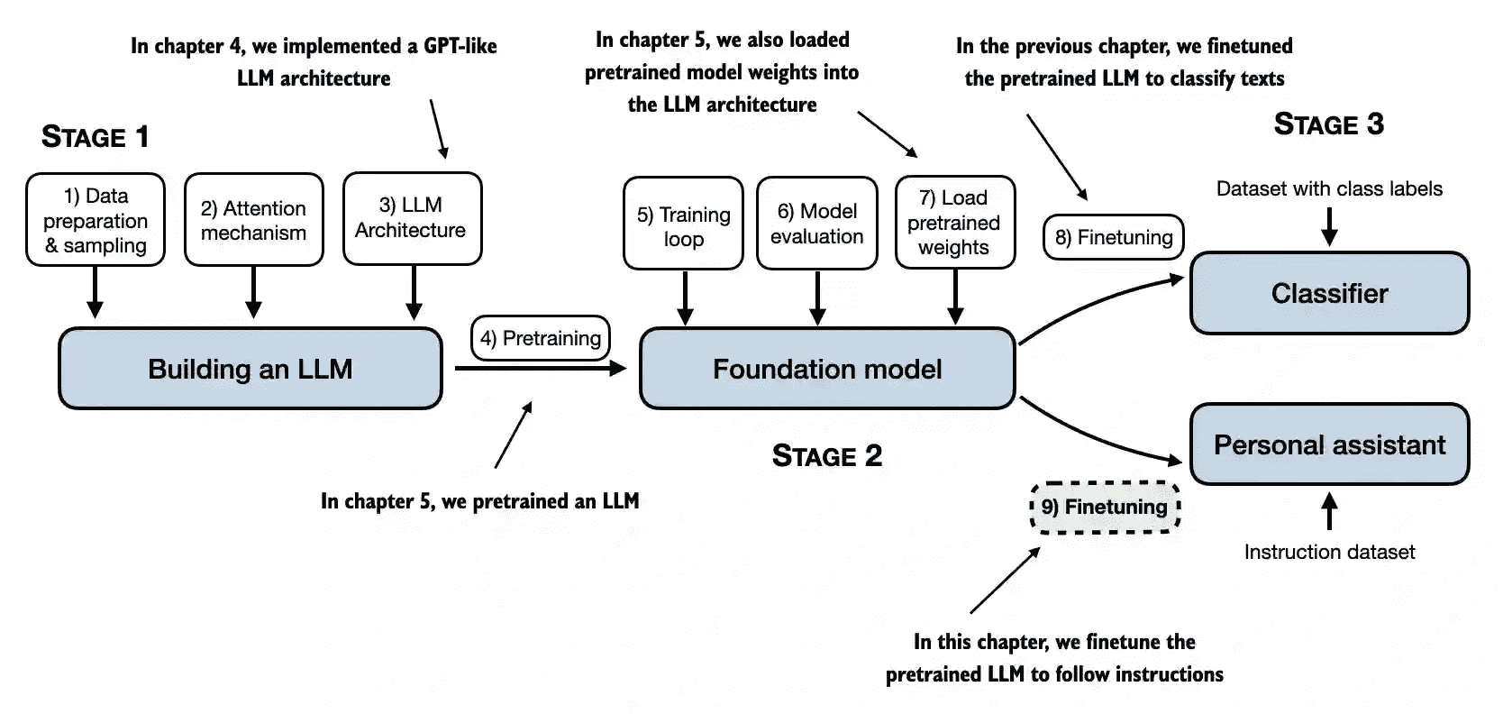
Figure 7.1 The three main stages of coding an LLM. This chapter focuses on step 9 of stage 3: fine-tuning a pretrained LLM to follow human instructions.
7.1 Introduction to instruction fine-tuning
instruction fine-tuning, also known as supervised instruction fine-tuning. Because it involves training a model on a dataset where the input-output pairs are explicitly provided
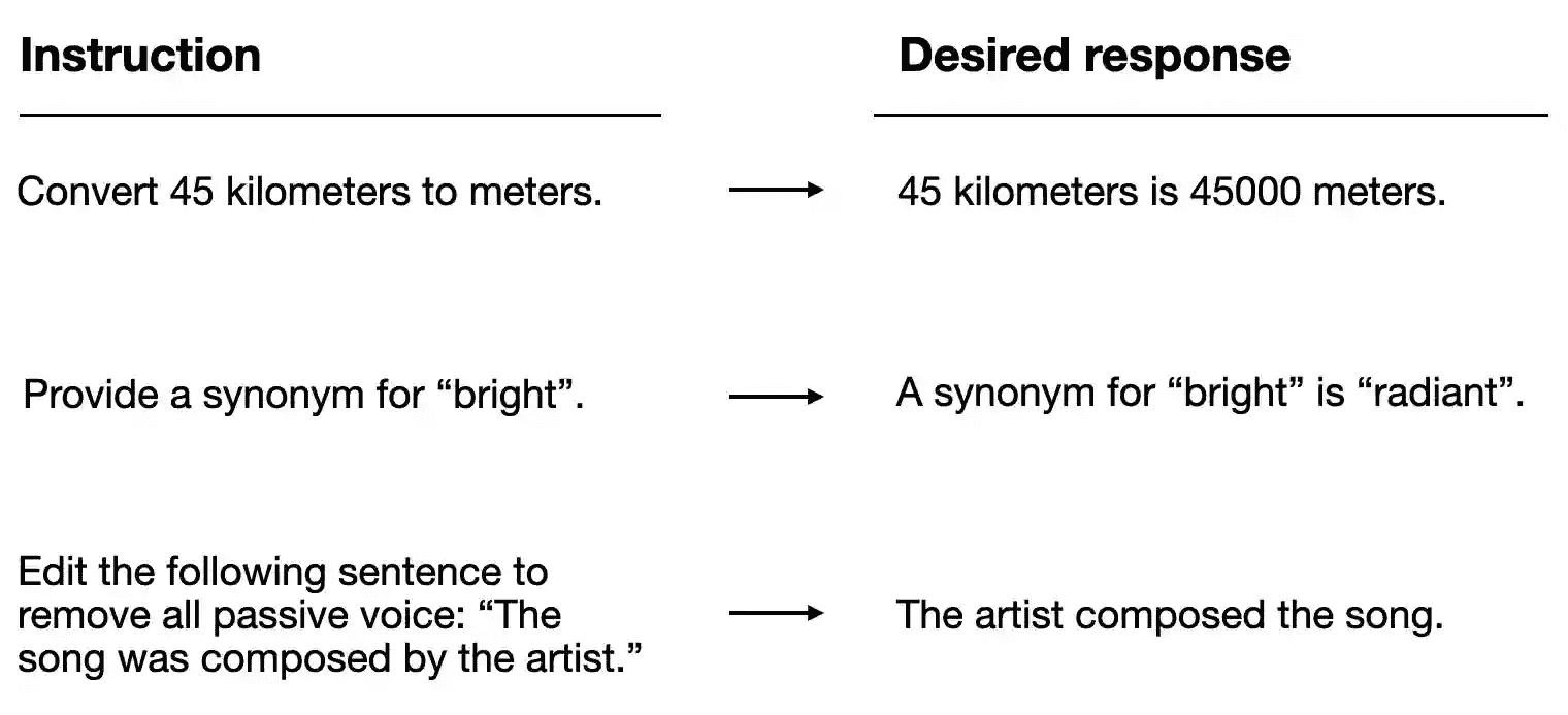
Figure 7.2 Examples of instructions that are processed by an LLM to generate desired responses
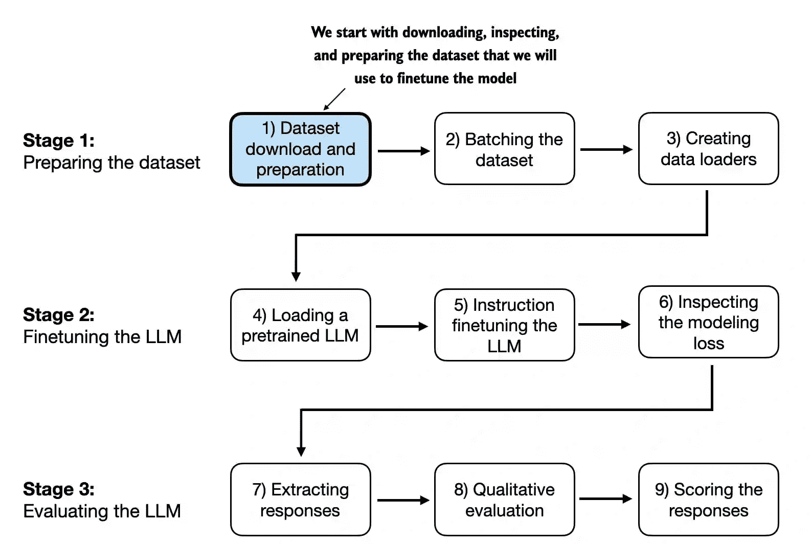
Figure 7.3 The three-stage process for instruction fine-tuning an LLM. Stage 1 involves dataset preparation, stage 2 focuses on model setup and fine-tuning, and stage 3 covers the evaluation of the model. We will begin with step 1 of stage 1: downloading and formatting the dataset.
7.2 Preparing a dataset for supervised instruction fine-tuning
There are different ways to format the entries as inputs to the LLM; the figure below illustrates two example formats that were used for training the Alpaca (https://crfm.stanford.edu/2023/03/13/alpaca.html) and Phi-3 (https://arxiv.org/abs/2404.14219) LLMs, respectively
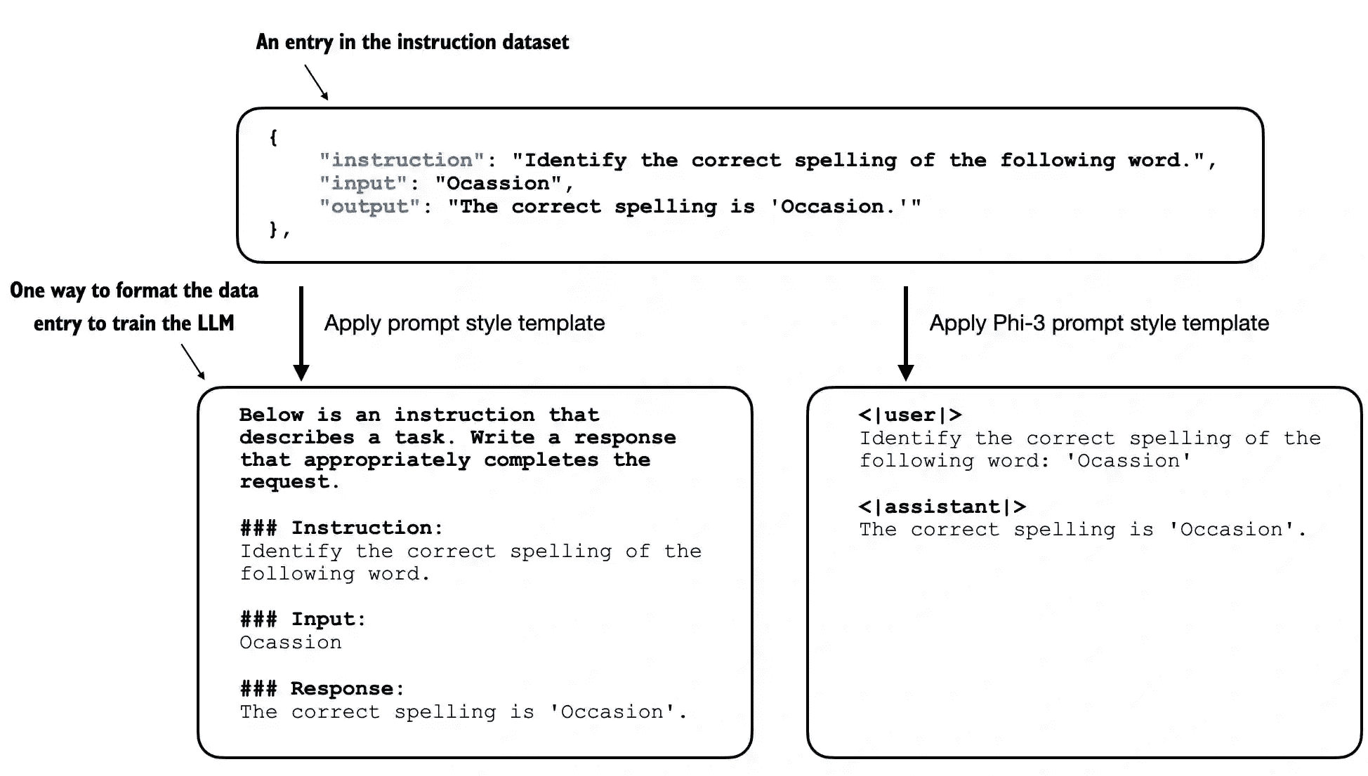
Figure 7.4 Comparison of prompt styles for instruction fine-tuning in LLMs. The Alpaca style (left) uses a structured format with defined sections for instruction, input, and response, while the Phi-3 style (right) employs a simpler format with designated <|user|> and <|assistant|> tokens.
prompt styles
Alpaca was one of the early LLMs to publicly detail its instruction fine-tuning process.
Phi-3, developed by Microsoft, is included to demonstrate the diversity in prompt styles.
备注
Fine-tuning the model with the Phi-3 template is approximately 17% faster than Alpaca template, since it results in shorter model inputs. The score is similar.
这儿用 Alpaca 格式的 prompt styles
下面代码是把数据转为 Alpaca 格式的代码
def format_input(entry):
    instruction_text = (
        f"Below is an instruction that describes a task. "
        f"Write a response that appropriately completes the request."
        f"\n\n### Instruction:\n{entry['instruction']}"
    )

    input_text = f"\n\n### Input:\n{entry['input']}" if entry["input"] else ""

    return instruction_text + input_text
7.3 Organizing data into training batches
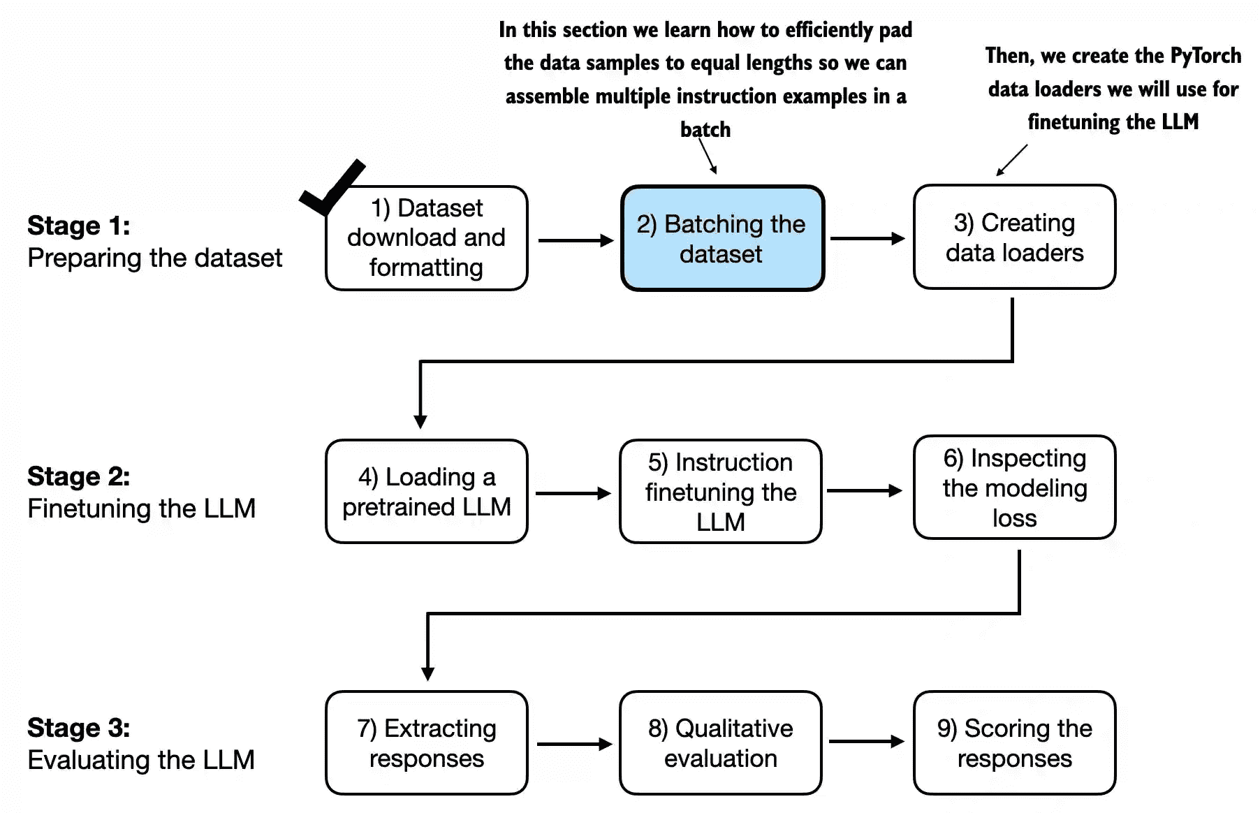
Figure 7.5 The three-stage process for instruction fine-tuning an LLM. Next, we look at step 2 of stage 1: assembling the training batches.
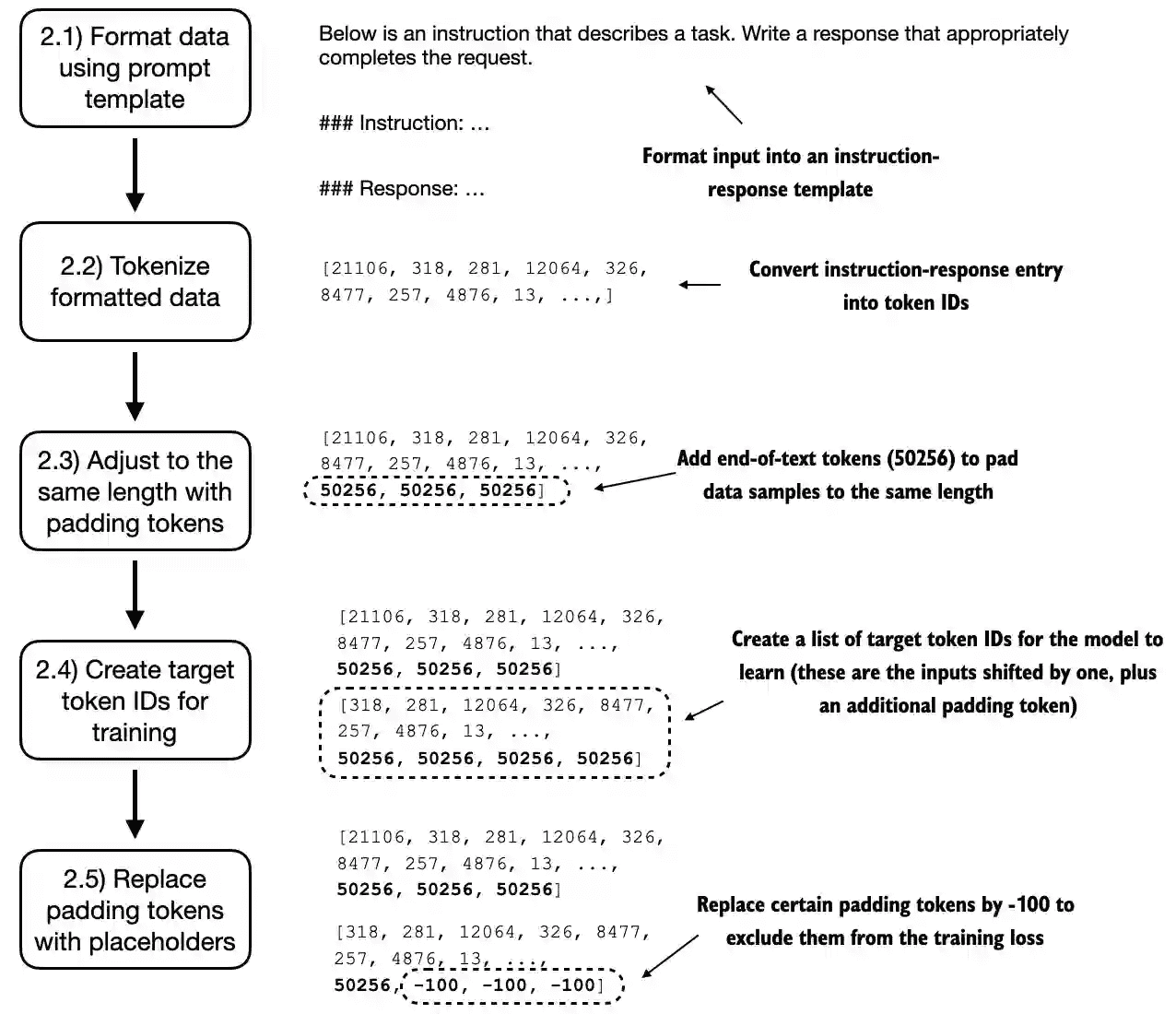
Figure 7.6 The five substeps involved in implementing the batching process: (2.1) applying the prompt template, (2.2) using tokenization from previous chapters, (2.3) adding padding tokens, (2.4) creating target token IDs, and (2.5) replacing -100 placeholder tokens to mask padding tokens in the loss function.
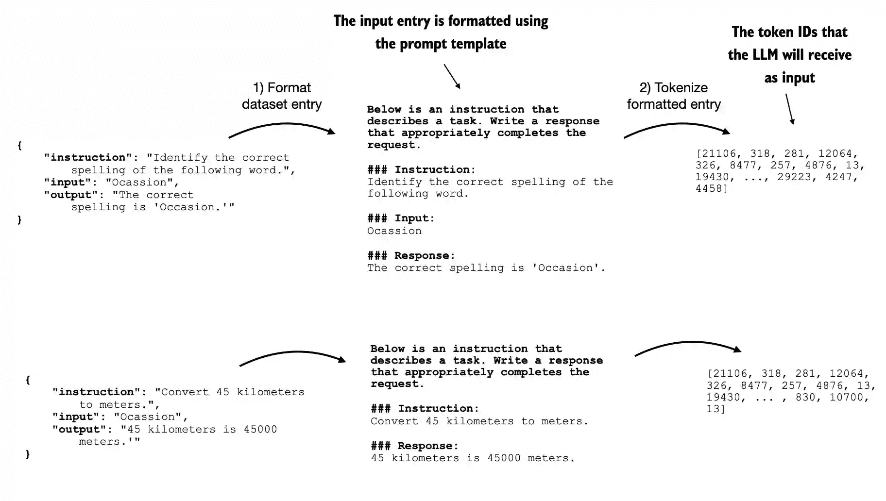
Figure 7.7 The first two steps involved in implementing the batching process. Entries are first formatted using a specific prompt template (2.1) and then tokenized (2.2), resulting in a sequence of token IDs that the model can process.
import torch
from torch.utils.data import Dataset


class InstructionDataset(Dataset):
    def __init__(self, data, tokenizer):
        self.data = data

        # Pre-tokenize texts
        self.encoded_texts = []
        for entry in data:
            instruction_plus_input = format_input(entry)
            response_text = f"\n\n### Response:\n{entry['output']}"
            full_text = instruction_plus_input + response_text
            self.encoded_texts.append(
                tokenizer.encode(full_text)
            )

    def __getitem__(self, index):
        return self.encoded_texts[index]

    def __len__(self):
        return len(self.data)
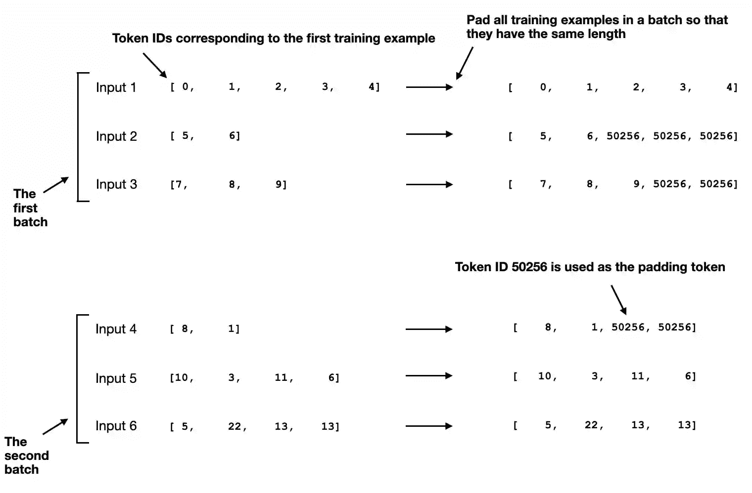
Figure 7.8 The padding of training examples in batches using token ID 50256 to ensure uniform length within each batch. Each batch may have different lengths, as shown by the first and second.
Here, we take a more sophisticated(优雅) approach and develop a custom “collate” function that we can pass to the data loader
This custom
collatefunction pads the training examples in each batch to have the same length (but different batches can have different lengths)
def custom_collate_draft_1(
    batch,
    pad_token_id=50256,
    device="cpu"
):
    # Find the longest sequence in the batch
    # and increase the max length by +1, which will add one extra
    # padding token below
    batch_max_length = max(len(item)+1 for item in batch)

    # Pad and prepare inputs
    inputs_lst = []

    for item in batch:
        new_item = item.copy()
        # Add an <|endoftext|> token
        new_item += [pad_token_id]
        # Pad sequences to batch_max_length
        padded = (
            new_item + [pad_token_id] * (batch_max_length - len(new_item))
        )
        # Via padded[:-1], we remove the extra padded token
        # that has been added via the +1 setting in batch_max_length
        # (the extra padding token will be relevant in later codes)
        inputs = torch.tensor(padded[:-1])
        inputs_lst.append(inputs)

    # Convert list of inputs to tensor and transfer to target device
    inputs_tensor = torch.stack(inputs_lst).to(device)
    return inputs_tensor
使用示例:
inputs_1 = [0, 1, 2, 3, 4]
inputs_2 = [5, 6]
inputs_3 = [7, 8, 9]

batch = (
    inputs_1,
    inputs_2,
    inputs_3
)

print(custom_collate_draft_1(batch))
# tensor([[    0,     1,     2,     3,     4],
#         [    5,     6, 50256, 50256, 50256],
#         [    7,     8,     9, 50256, 50256]])
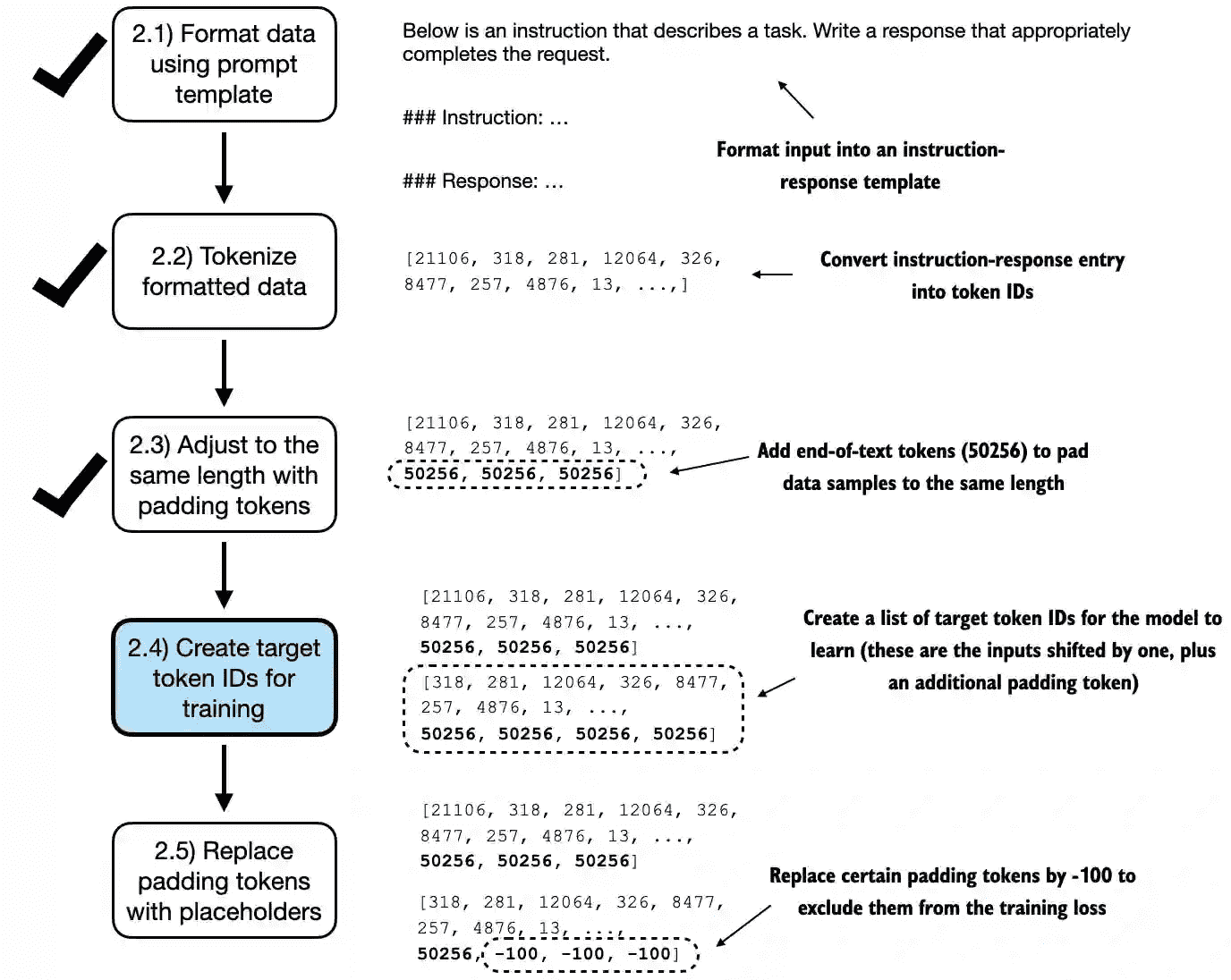
Figure 7.9 The five substeps involved in implementing the batching process. We are now focusing on step 2.4, the creation of target token IDs. This step is essential as it
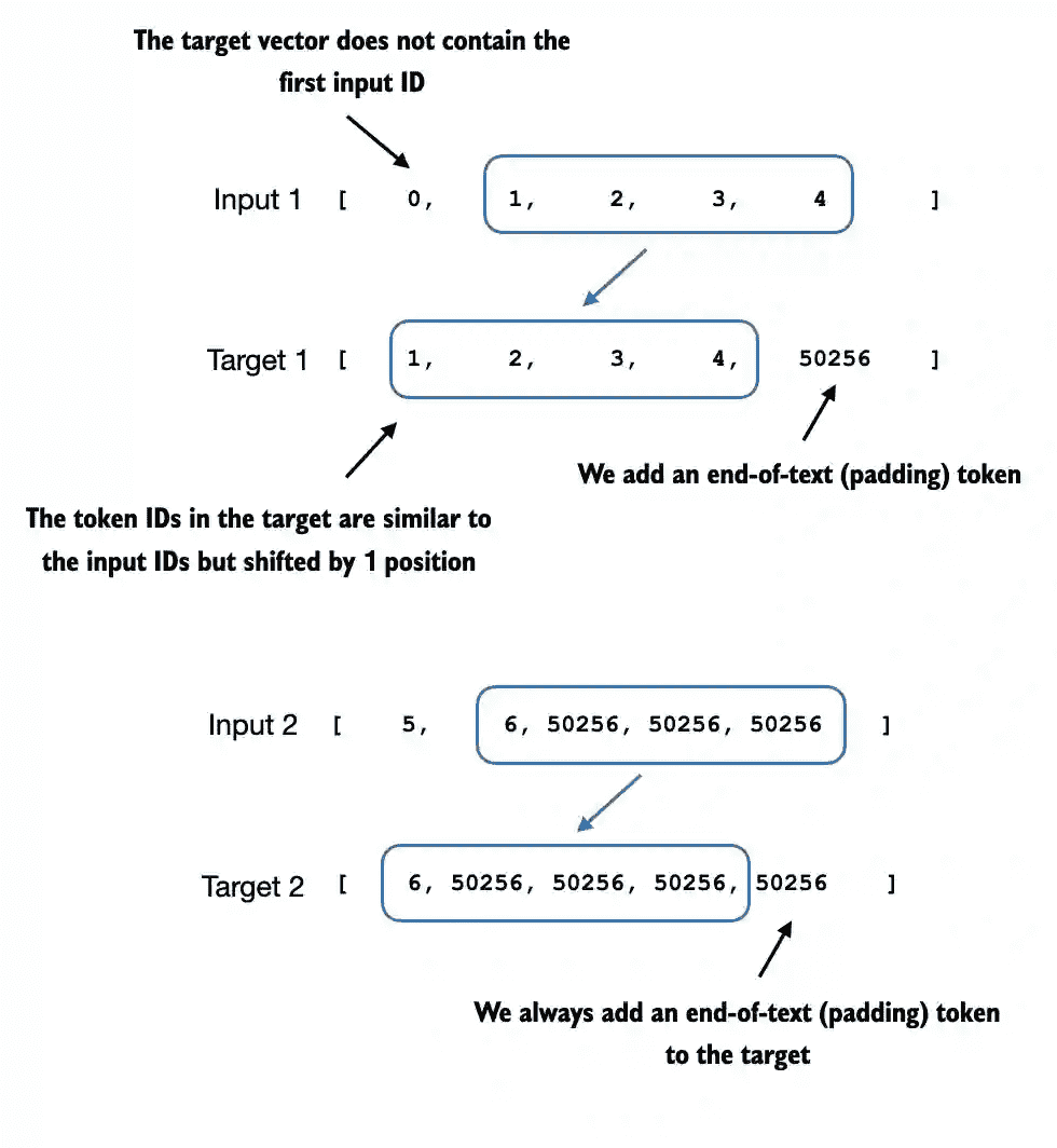
Figure 7.10 The input and target token alignment used in the instruction fine-tuning process of an LLM. For each input sequence, the corresponding target sequence is created by shifting the token IDs one position to the right, omitting the first token of the input, and appending an end-of-text token.
def custom_collate_draft_2(
    batch,
    pad_token_id=50256,
    device="cpu"
):
    # Find the longest sequence in the batch
    batch_max_length = max(len(item)+1 for item in batch)

    # Pad and prepare inputs
    inputs_lst, targets_lst = [], []

    for item in batch:
        new_item = item.copy()
        # Add an <|endoftext|> token
        new_item += [pad_token_id]
        # Pad sequences to max_length
        padded = (
            new_item + [pad_token_id] *
            (batch_max_length - len(new_item))
        )
        inputs = torch.tensor(padded[:-1])  # Truncate the last token for inputs
        targets = torch.tensor(padded[1:])  # Shift +1 to the right for targets⭕️
        inputs_lst.append(inputs)
        targets_lst.append(targets)

    # Convert list of inputs to tensor and transfer to target device
    inputs_tensor = torch.stack(inputs_lst).to(device)
    targets_tensor = torch.stack(targets_lst).to(device)
    return inputs_tensor, targets_tensor
使用示例:
inputs, targets = custom_collate_draft_2(batch)
print(inputs)
print(targets)
# tensor([[    0,     1,     2,     3,     4],
#         [    5,     6, 50256, 50256, 50256],
#         [    7,     8,     9, 50256, 50256]])
# tensor([[    1,     2,     3,     4, 50256],
#         [    6, 50256, 50256, 50256, 50256],
#         [    8,     9, 50256, 50256, 50256]])
Next, we introduce an
ignore_indexvalue to replace all padding token IDs with a new value; the purpose of thisignore_indexis that we can ignore padding values in the loss function (more on that later)This special value allows us to exclude these padding tokens from contributing to the training loss calculation, ensuring that only meaningful data influences model learning.
We will discuss this process in more detail after we implement this modification. (When fine-tuning for classification, we did not have to worry about this since we only trained the model based on the last output token.)
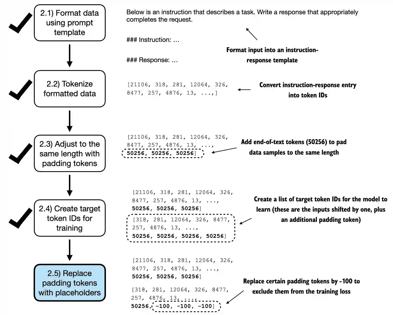
Figure 7.11 The five substeps involved in implementing the batching process. After creating the target sequence by shifting token IDs one position to the right and appending an end-of-text token, in step 2.5, we replace the end-of-text padding tokens with a placeholder value ( -100 ).
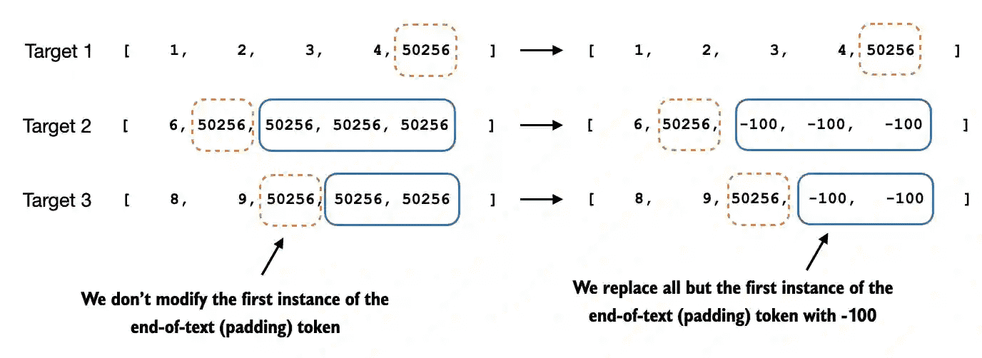
Figure 7.12 Step 2.4 in the token replacement process in the target batch for the training data preparation. We replace all but the first instance of the end-of-text token, which we use as padding, with the placeholder value -100 , while keeping the initial end-of-text token in each target sequence.
def custom_collate_fn(
    batch,
    pad_token_id=50256,
    ignore_index=-100,
    allowed_max_length=None,
    device="cpu"
):
    # Find the longest sequence in the batch
    batch_max_length = max(len(item)+1 for item in batch)

    # Pad and prepare inputs and targets
    inputs_lst, targets_lst = [], []

    for item in batch:
        new_item = item.copy()
        # Add an <|endoftext|> token
        new_item += [pad_token_id]
        # Pad sequences to max_length
        padded = (
            new_item + [pad_token_id] *
            (batch_max_length - len(new_item))
        )
        inputs = torch.tensor(padded[:-1])  # Truncate the last token for inputs
        targets = torch.tensor(padded[1:])  # Shift +1 to the right for targets

        # New: Replace all but the first padding tokens in targets by ignore_index
        mask = targets == pad_token_id
        indices = torch.nonzero(mask).squeeze()
        if indices.numel() > 1:
            targets[indices[1:]] = ignore_index

        # New: Optionally truncate to maximum sequence length
        if allowed_max_length is not None:
            inputs = inputs[:allowed_max_length]
            targets = targets[:allowed_max_length]

        inputs_lst.append(inputs)
        targets_lst.append(targets)

    # Convert list of inputs and targets to tensors and transfer to target device
    inputs_tensor = torch.stack(inputs_lst).to(device)
    targets_tensor = torch.stack(targets_lst).to(device)

    return inputs_tensor, targets_tensor
使用示例:
inputs, targets = custom_collate_fn(batch)
print(inputs)
print(targets)

# tensor([[    0,     1,     2,     3,     4],
#         [    5,     6, 50256, 50256, 50256],
#         [    7,     8,     9, 50256, 50256]])
# tensor([[    1,     2,     3,     4, 50256],
#         [    6, 50256,  -100,  -100,  -100],
#         [    8,     9, 50256,  -100,  -100]])
why replacement by -100
Let’s see what this replacement by -100 accomplishes
For illustration purposes, let’s assume we have a small classification task with 2 class labels, 0 and 1, similar to chapter 6
If we have the following logits values (outputs of the last layer of the model), we calculate the following loss
示例1:
logits_1 = torch.tensor(
    [[-1.0, 1.0],  # 1st training example
     [-0.5, 1.5]]  # 2nd training example
)
targets_1 = torch.tensor([0, 1])


loss_1 = torch.nn.functional.cross_entropy(logits_1, targets_1)
print(loss_1)
# tensor(1.1269)
Now, adding one more training example will, as expected, influence the loss:
logits_2 = torch.tensor(
    [[-1.0, 1.0],
     [-0.5, 1.5],
     [-0.5, 1.5]]  # New 3rd training example
)
targets_2 = torch.tensor([0, 1, 1])

loss_2 = torch.nn.functional.cross_entropy(logits_2, targets_2)
print(loss_2)
# tensor(0.7936)
Let’s see what happens if we replace the class label of one of the examples with -100:
targets_3 = torch.tensor([0, 1, -100])

loss_3 = torch.nn.functional.cross_entropy(logits_2, targets_3)
print(loss_3)
print("loss_1 == loss_3:", loss_1 == loss_3)
# tensor(1.1269)
# loss_1 == loss_3: tensor(True)
As we can see, the resulting loss on these 3 training examples is the same as the loss we calculated from the 2 training examples, which means that the cross-entropy loss function ignored the training example with the -100 label
By default, PyTorch has the
cross_entropy(..., ignore_index=-100)setting to ignore examples corresponding to the label -100Using this -100
ignore_index, we can ignore the additional end-of-text (padding) tokens in the batches that we used to pad the training examples to equal lengthHowever, we don’t want to ignore the first instance of the end-of-text (padding) token (50256) because it can help signal to the LLM when the response is complete
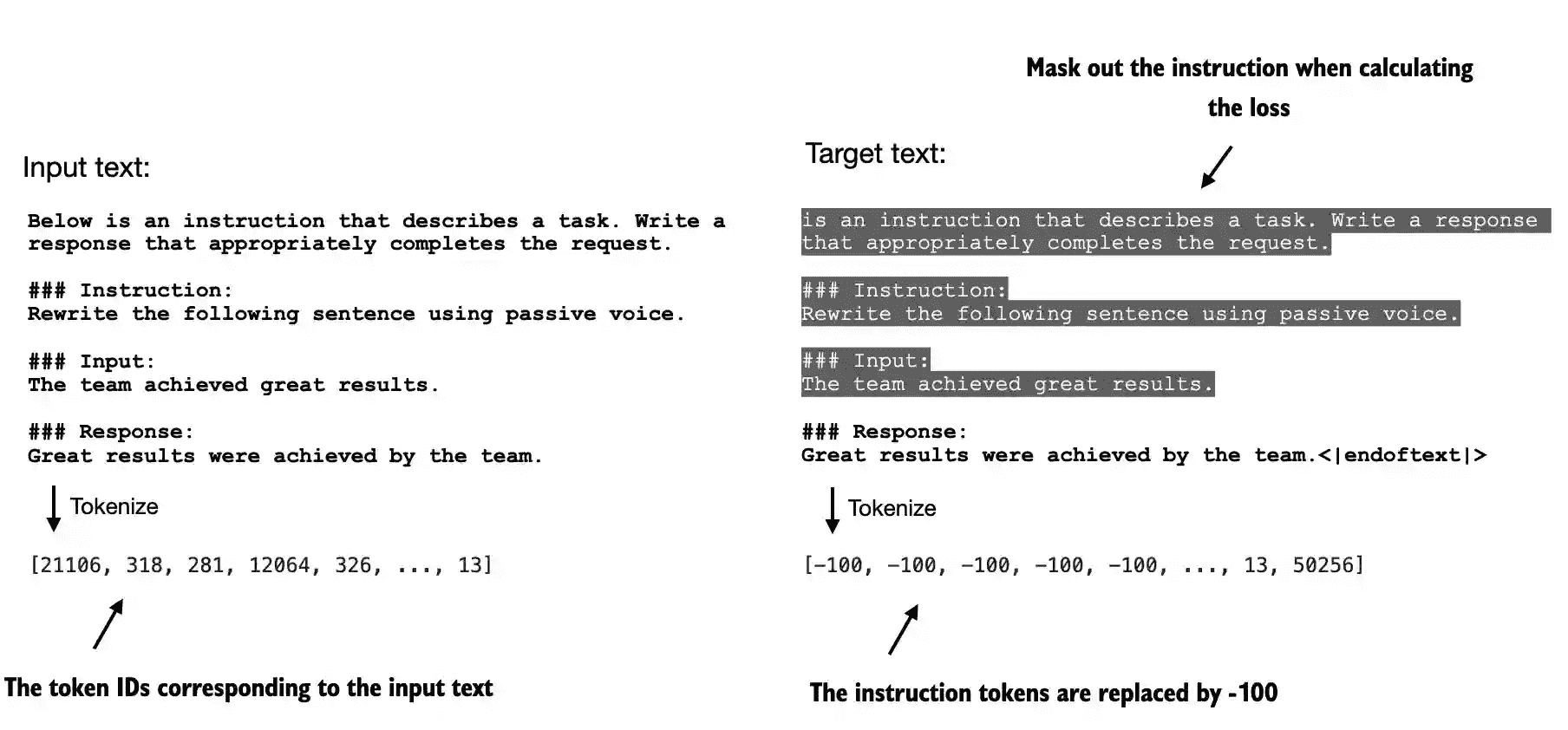
Figure 7.13 Left: The formatted input text we tokenize and then feed to the LLM during training. Right: The target text we prepare for the LLM where we can optionally mask out the instruction section, which means replacing the corresponding token IDs with -100 ignore_index the value.
备注
As of this writing, researchers are divided on whether masking the instructions is universally beneficial during instruction fine- tuning. For instance, the 2024 paper by Shi et al., “Instruction Tuning With Loss Over Instructions” (https://arxiv.org/abs/2405.14394), demonstrated that not masking the instructions benefits the LLM performance (see appendix B for more details).
7.4 Creating data loaders for an instruction dataset
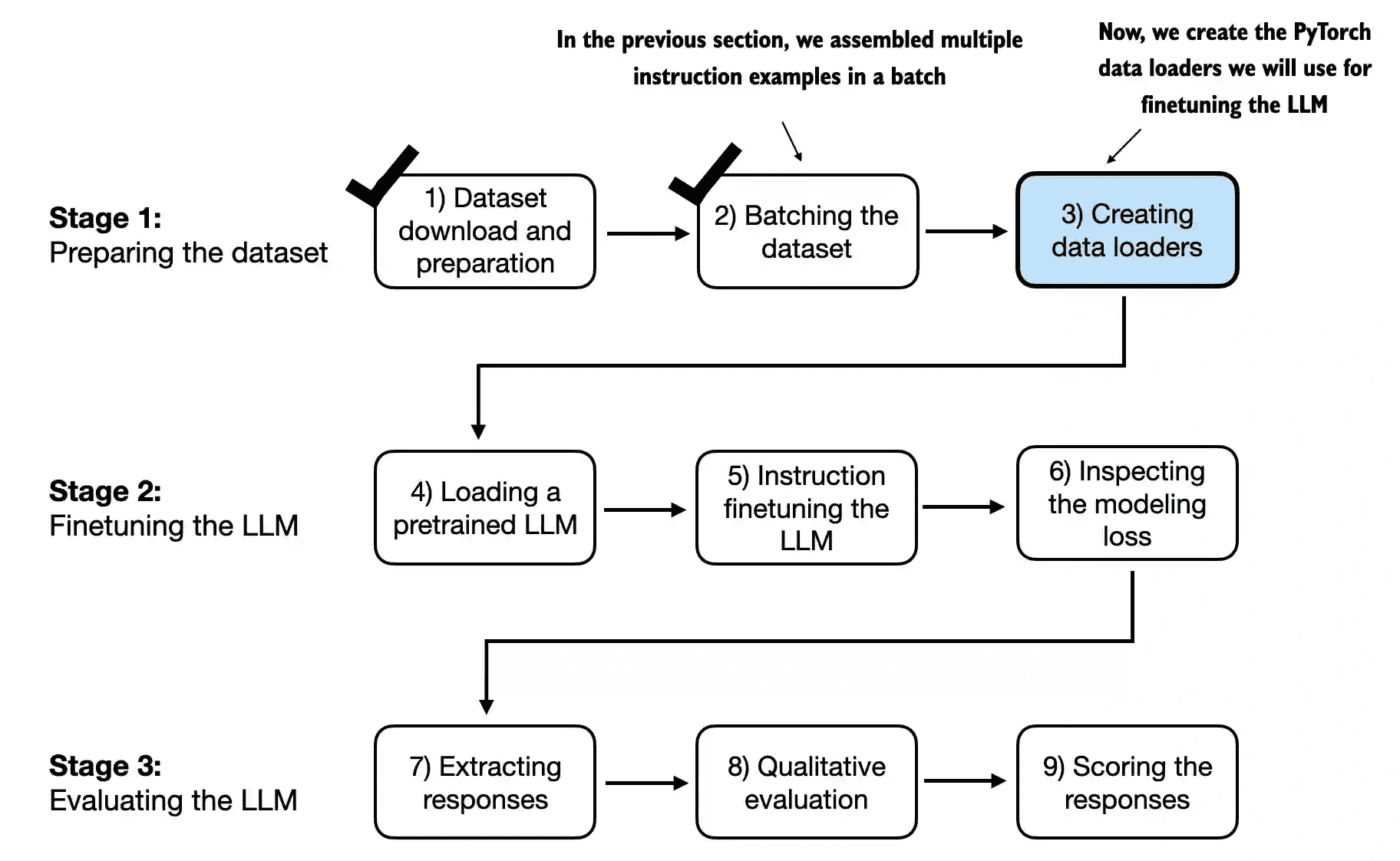
Figure 7.14 The three-stage process for instruction fine-tuning an LLM. Thus far, we have prepared the dataset and implemented a custom collate function to batch the instruction dataset. Now, we can create and apply the data loaders to the training, validation, and test sets needed for the LLM instruction fine-tuning and evaluation.
Instantiate the data loaders similar to previous chapters, except that we now provide our own collate function for the batching process
from functools import partial

customized_collate_fn = partial(
    custom_collate_fn,
    device=device,
    allowed_max_length=1024
)

from torch.utils.data import DataLoader


num_workers = 0
batch_size = 8

torch.manual_seed(123)

train_dataset = InstructionDataset(train_data, tokenizer)
train_loader = DataLoader(
    train_dataset,
    batch_size=batch_size,
    collate_fn=customized_collate_fn,
    shuffle=True,
    drop_last=True,
    num_workers=num_workers
)
... ... # 验证集、测试集相同
应用:
print("Train loader:")
for inputs, targets in train_loader:
    print(inputs.shape, targets.shape)
# 输出
Train loader:
#  8 represents the batch size and 61 is the number of tokens in each training example in this batch.
torch.Size([8, 61]) torch.Size([8, 61])   # 批次: 8, 本批次最长:61
torch.Size([8, 76]) torch.Size([8, 76])   # 批次: 8, 本批次最长:76
... ...
torch.Size([8, 66]) torch.Size([8, 66])   # ...
torch.Size([8, 74]) torch.Size([8, 74])
torch.Size([8, 69]) torch.Size([8, 69])
print(inputs[0]):
tensor([21106,   318,   281, 12064,   326,  8477,   257,  4876,    13, 19430,
          257,  2882,   326, 20431, 32543,   262,  2581,    13,   198,   198,
        21017, 46486,    25,   198, 30003,  6525,   262,  6827,  1262,   257,
          985,   576,    13,   198,   198, 21017, 23412,    25,   198,   464,
         5156,   318,   845, 13779,    13,   198,   198, 21017, 18261,    25,
          198,   464,  5156,   318,   355, 13779,   355,   257,  4936,    13,
        50256, 50256, 50256, 50256, 50256, 50256, 50256, 50256, 50256],
       device='cuda:0')
print(targets[0]):
tensor([  318,   281, 12064,   326,  8477,   257,  4876,    13, 19430,   257,
         2882,   326, 20431, 32543,   262,  2581,    13,   198,   198, 21017,
        46486,    25,   198, 30003,  6525,   262,  6827,  1262,   257,   985,
          576,    13,   198,   198, 21017, 23412,    25,   198,   464,  5156,
          318,   845, 13779,    13,   198,   198, 21017, 18261,    25,   198,
          464,  5156,   318,   355, 13779,   355,   257,  4936,    13, 50256,
         -100,  -100,  -100,  -100,  -100,  -100,  -100,  -100,  -100],
       device='cuda:0')
7.5 Loading a pretrained LLM
备注
Instead of using the smallest 124-million-parameter model as before, we load the medium-sized model with 355 million parameters. The reason for this choice is that the 124-million- parameter model is too limited in capacity to achieve satisfactory results via instruction fine-tuning. Specifically, smaller models lack the necessary capacity to learn and retain the intricate patterns and nuanced behaviors required for high- quality instruction-following tasks.
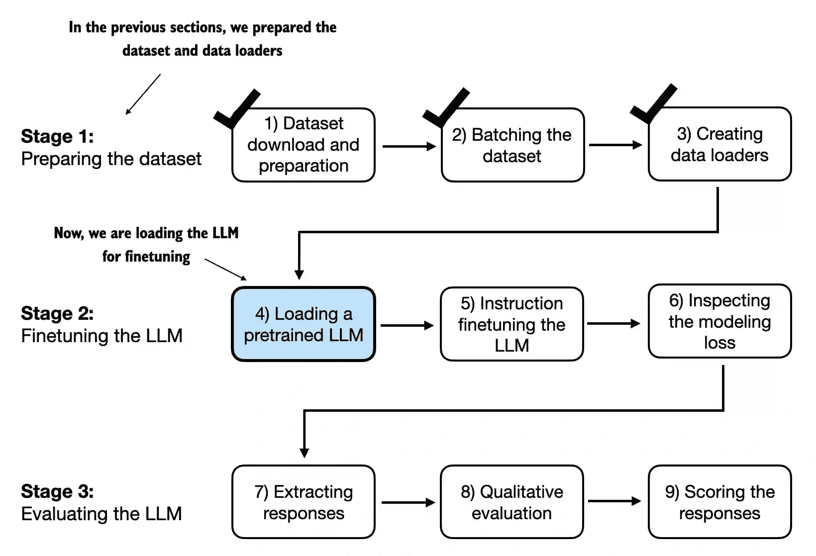
Figure 7.15 The three-stage process for instruction fine- tuning an LLM. After the dataset preparation, the process of fine-tuning an LLM for instruction-following begins with loading a pretrained LLM, which serves as the foundation for subsequent training.
7.6 Fine-tuning the LLM on instruction data
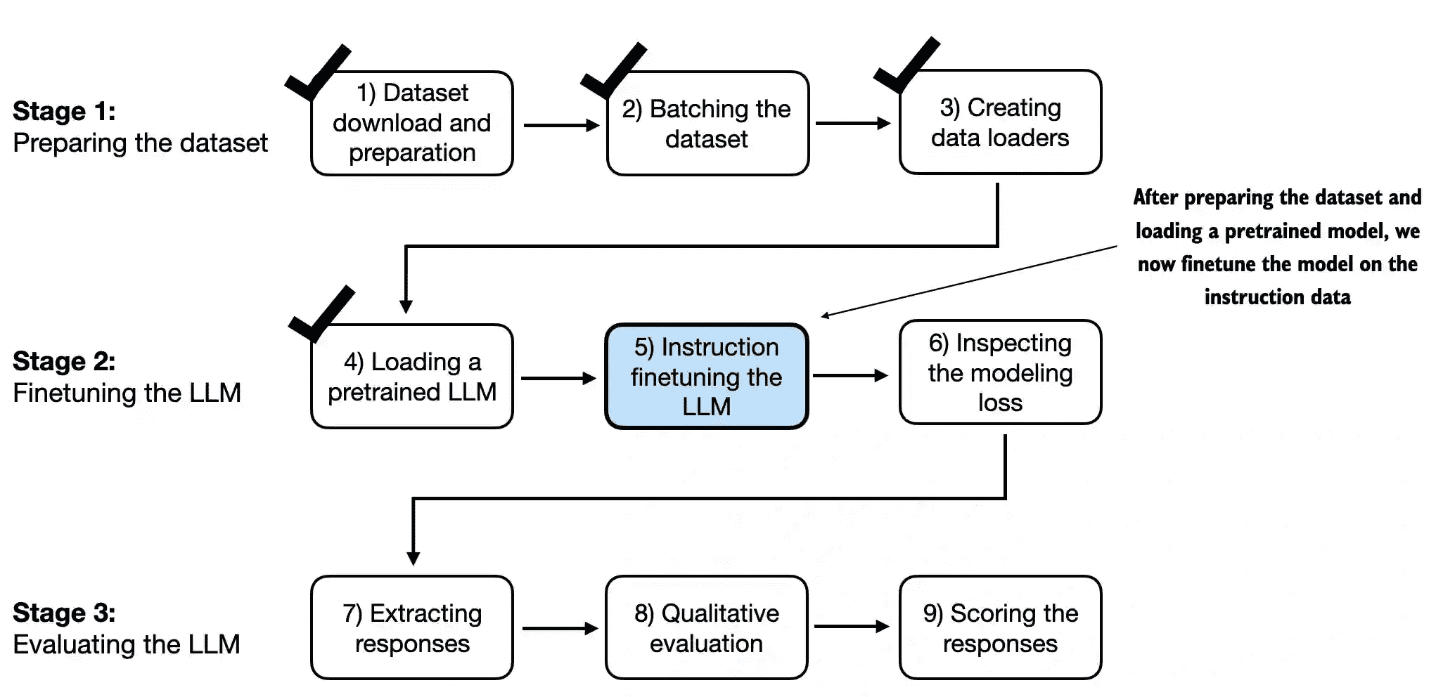
Figure 7.16 The three-stage process for instruction fine- tuning an LLM. In step 5, we train the pretrained model we previously loaded on the instruction dataset we prepared earlier.
7.7 Extracting and saving responses
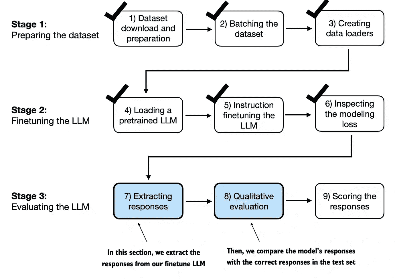
Figure 7.18 The three-stage process for instruction fine- tuning the LLM. In the first two steps of stage 3, we extract and collect the model responses on the held-out test dataset for further analysis and then evaluate the model to quantify the performance of the instruction-fine-tuned LLM.
- In practice, instruction-fine-tuned LLMs such as chatbots are evaluated via multiple approaches:
Short-answer and multiple-choice benchmarks, such as Measuring Massive Multitask Language Understanding (MMLU; https://arxiv.org/abs/2009.03300), which test the general knowledge of a model.
Human preference comparison to other LLMs, such as LMSYS chatbot arena (https://arena.lmsys.org).
Automated conversational benchmarks, where another LLM like GPT-4 is used to evaluate the responses, such as AlpacaEval (https://tatsu-lab.github.io/alpaca_eval/).
本文将使用第3种方法(AlpacaEval)
先把输入、期望输出和模型输出数据整理出来
from tqdm import tqdm

for i, entry in tqdm(enumerate(test_data), total=len(test_data)):

    input_text = format_input(entry)

    token_ids = generate(
        model=model,
        idx=text_to_token_ids(input_text, tokenizer).to(device),
        max_new_tokens=256,
        context_size=BASE_CONFIG["context_length"],
        eos_id=50256
    )
    generated_text = token_ids_to_text(token_ids, tokenizer)
    response_text = generated_text[len(input_text):].replace("### Response:", "").strip()

    test_data[i]["model_response"] = response_text


with open("instruction-data-with-response.json", "w") as file:
    json.dump(test_data, file, indent=4)  # "indent" for pretty-printing
7.8 Evaluating the fine-tuned LLM
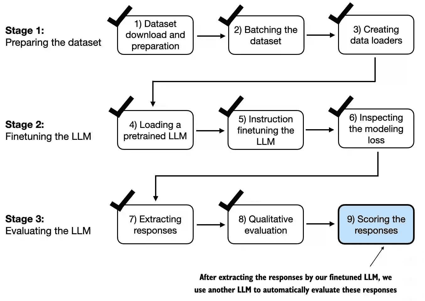
Figure 7.19 The three-stage process for instruction fine-tuning the LLM. In this last step of the instruction-fine-tuning pipeline, we implement a method to quantify the performance of the fine-tuned model by scoring the responses it generated for the test.
def format_input(entry):
    instruction_text = (
        f"Below is an instruction that describes a task. "
        f"Write a response that appropriately completes the request."
        f"\n\n### Instruction:\n{entry['instruction']}"
    )

    input_text = f"\n\n### Input:\n{entry['input']}" if entry["input"] else ""

    return instruction_text + input_text

for entry in test_data[:3]:
    prompt = (
        f"Given the input `{format_input(entry)}` "
        f"and correct output `{entry['output']}`, "
        f"score the model response `{entry['model_response']}`"
        f" on a scale from 0 to 100, where 100 is the best score. "
    )
    print("\nDataset response:")
    print(">>", entry['output'])
    print("\nModel response:")
    print(">>", entry["model_response"])
    print("\nScore:")
    print(">>", query_model(prompt))
    print("\n-------------------------")
# 输出
Dataset response:
>> The car is as fast as lightning.

Model response:
>> The car is as fast as a bullet.

Score:
>> I'd rate the model response "The car is as fast as a bullet." an 85 out of 100.
只显示百分比数字的prompt:
prompt = (
    f"Given the input `{format_input(entry)}` "
    f"and correct output `{entry['output']}`, "
    f"score the model response `{entry[json_key]}`"
    f" on a scale from 0 to 100, where 100 is the best score. "
    f"Respond with the integer number only."        # added ❇️
)
7.9 Conclusions
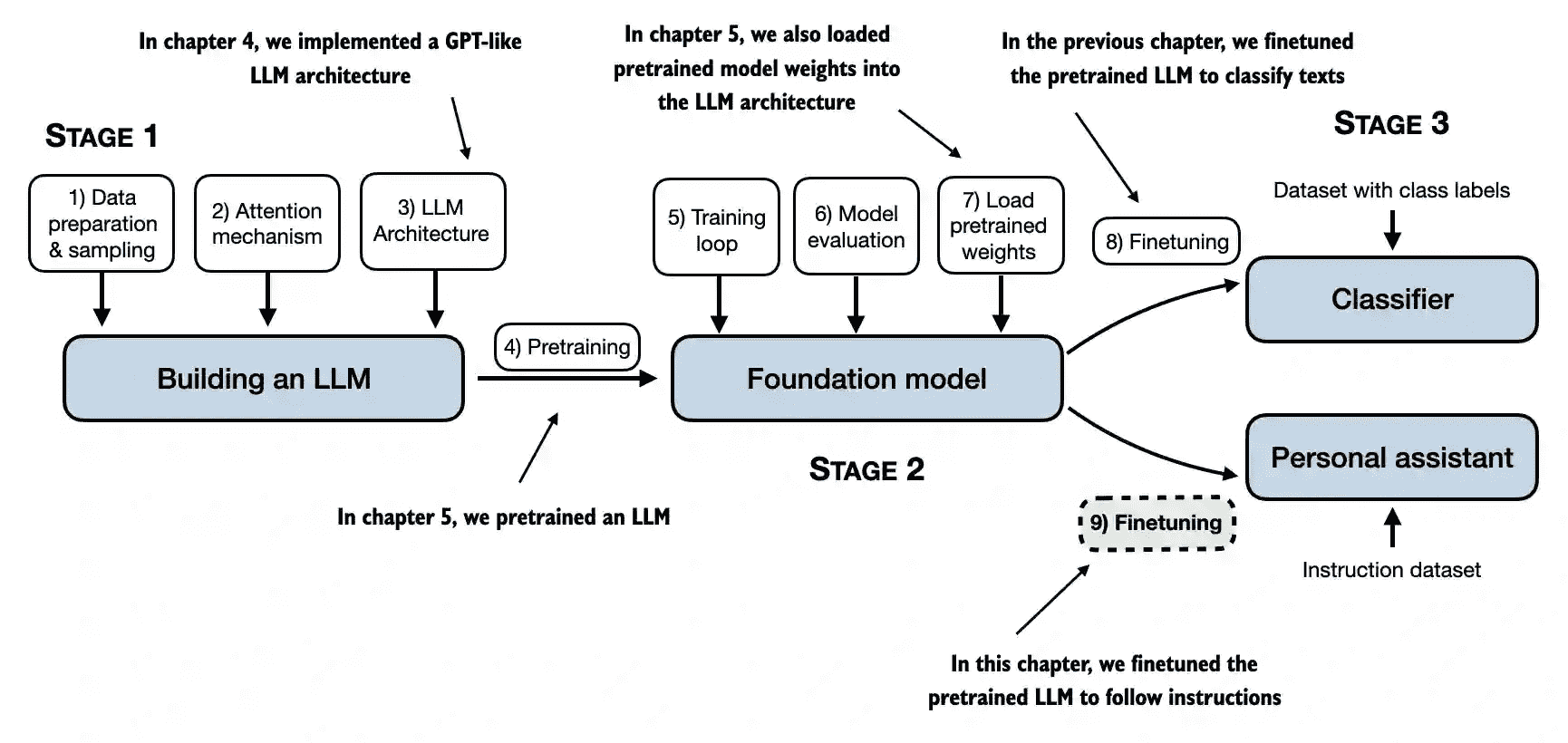
Figure 7.21 The three main stages of coding an LLM.
While we covered the most essential steps, there is an optional step that can be performed after instruction fine-tuning:
preference fine-tuning.Preference fine-tuningis particularly useful for customizing a model to better align with specific user preferences.
Summary
The instruction-fine-tuning process adapts a pretrained LLM to follow human instructions and generate desired responses.
Preparing the dataset involves downloading an instruction-response dataset, formatting the entries, and splitting it into train, validation, and test sets.
Training batches are constructed using a custom collate function that pads sequences, creates target token IDs, and masks padding tokens.
We load a pretrained GPT-2 medium model with 355 million parameters to serve as the starting point for instruction fine-tuning.
The pretrained model is fine-tuned on the instruction dataset using a training loop similar to pretraining.
Evaluation involves extracting model responses on a test set and scoring them (for example, using another LLM).
The Ollama application with an 8-billion-parameter Llama model can be used to automatically score the fine-tuned model’s responses on the test set, providing an average score to quantify performance.
Appendix A. Introduction to PyTorch
A.1 What is PyTorch
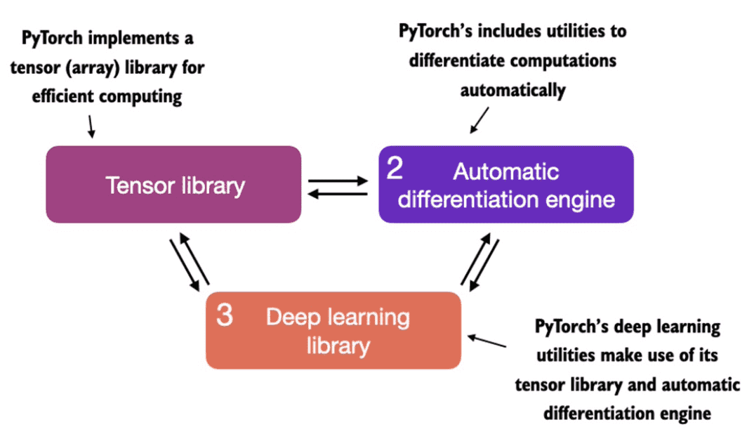
Figure A.1 PyTorch’s three main components include a tensor library as a fundamental building block for computing, automatic differentiation for model optimization, and deep learning utility functions, making it easier to implement and train deep neural network models.
Firstly, PyTorch is a tensor library that extends the concept of array-oriented programming library NumPy with the additional feature of accelerated computation on GPUs, thus providing a seamless switch between CPUs and GPUs.
Secondly, PyTorch is an automatic differentiation engine, also known as autograd, which enables the automatic computation of gradients for tensor operations, simplifying backpropagation and model optimization.
Finally, PyTorch is a deep learning library, meaning that it offers modular, flexible, and efficient building blocks (including pre-trained models, loss functions, and optimizers) for designing and training a wide range of deep learning models, catering to both researchers and developers.
A.2 Understanding tensors
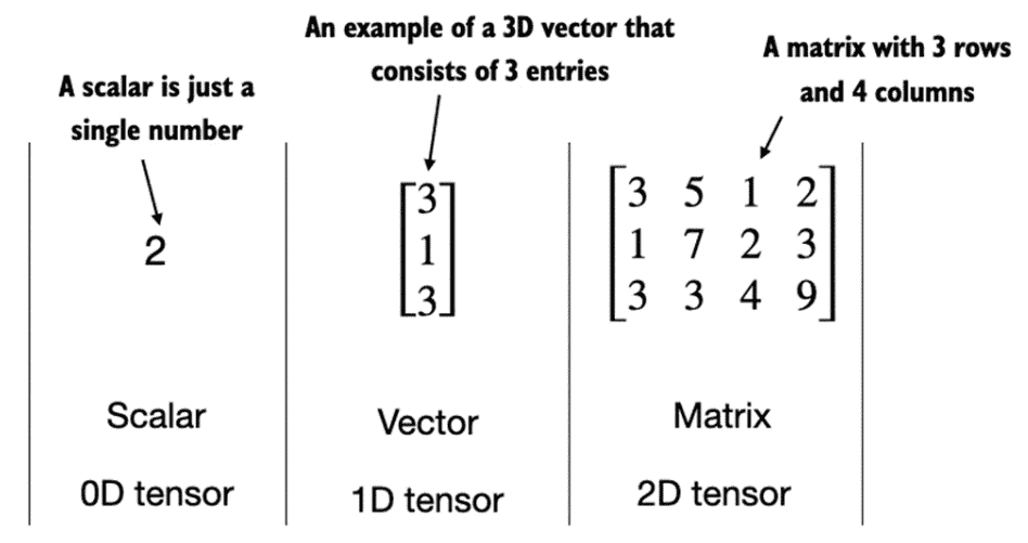
Figure A.6 An illustration of tensors with different ranks. Here 0D corresponds to rank 0, 1D to rank 1, and 2D to rank 2. Note that a 3D vector, which consists of 3 elements, is still a rank 1 tensor.
PyTorch’s has a NumPy-like API
A.3 Seeing models as computation graphs
Automatic differentiation engine, also known as autograd. PyTorch’s autograd system provides functions to compute gradients in dynamic computational graphs automatically.
Computation graph is a directed graph that allows us to express and visualize mathematical expressions.
In the context of deep learning, a computation graph lays out the sequence of calculations needed to compute the output of a neural network – we will need this later to compute the required gradients for backpropagation, which is the main training algorithm for neural networks.
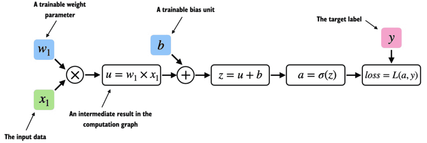
Figure A.7 A logistic regression forward pass as a computation graph. The input feature x1 is multiplied by a model weight w1 and passed through an activation function σ after adding the bias. The loss is computed by comparing the model output a with a given label y.
In fact, PyTorch builds such a computation graph in the background, and we can use this to calculate gradients of a loss function with respect to the model parameters (here w1 and b) to train the model
A.4 Automatic differentiation made easy
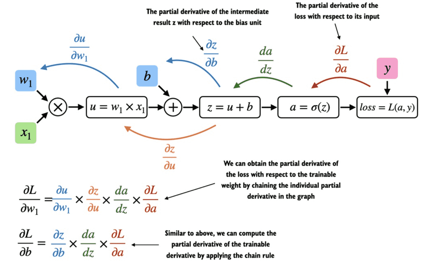
Figure A.8 The most common way of computing the loss gradients in a computation graph involves applying the chain rule from right to left, which is also called reverse-model automatic differentiation or backpropagation. It means we start from the output layer (or the loss itself) and work backward through the network to the input layer. This is done to compute the gradient of the loss with respect to each parameter (weights and biases) in the network, which informs how we update these parameters during training.
Gradients are required when training neural networks via the popular backpropagation algorithm, which can be thought of as an implementation of the chain rule from calculus for neural networks
Partial derivatives and gradients
A partial derivatives, which measure the rate at which a function changes with respect to one of its variables.
A gradient is a vector containing all of the partial derivatives of a multivariate function, a function with more than one variable as input.
This provides the information needed to update each parameter in a way that minimizes the loss function, which serves as a proxy for measuring the model’s performance, using a method such as gradient descent.
Listing A.3 Computing gradients via autograd
import torch.nn.functional as F
from torch.autograd import grad
y = torch.tensor([1.0])
x1 = torch.tensor([1.1])
w1 = torch.tensor([2.2], requires_grad=True)
b = torch.tensor([0.0], requires_grad=True)
z = x1 * w1 + b
a = torch.sigmoid(z)

loss = F.binary_cross_entropy(a, y)
grad_L_w1 = grad(loss, w1, retain_graph=True)  #A
grad_L_b = grad(loss, b, retain_graph=True)
PyTorch provides even more high-level tools to automate this process:
loss.backward()
print(w1.grad)
print(b.grad)
A.5 Implementing multilayer neural networks
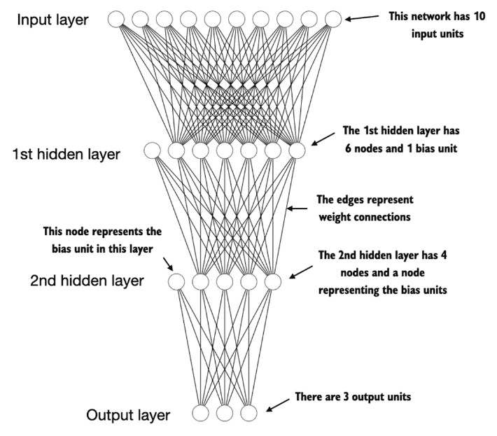
Figure A.9 An illustration of a multilayer perceptron with 2 hidden layers. Each node represents a unit in the respective layer. Each layer has only a very small number of nodes for illustration purposes.
Listing A.4 A multilayer perceptron with two hidden layers
class NeuralNetwork(torch.nn.Module):
    def __init__(self, num_inputs, num_outputs):  #A
        super().__init__()
        self.layers = torch.nn.Sequential(
            # 1st hidden layer
            torch.nn.Linear(num_inputs, 30),  #B
            torch.nn.ReLU(),  #C
            # 2nd hidden layer
            torch.nn.Linear(30, 20),  #D
            torch.nn.ReLU(),
            # output layer
            torch.nn.Linear(20, num_outputs),
        )
    def forward(self, x):
        logits = self.layers(x)
        return logits   #E
instantiate a new neural network object:
>>> model = NeuralNetwork(50, 3)
NeuralNetwork(
  (layers): Sequential(
    (0): Linear(in_features=50, out_features=30, bias=True)
    (1): ReLU()
    (2): Linear(in_features=30, out_features=20, bias=True)
    (3): ReLU()
    (4): Linear(in_features=20, out_features=3, bias=True)
  )
)
check the total number of trainable parameters:
>>> sum(p.numel() for p in model.parameters() if p.requires_grad)
2213

手动计算:
第一个隐藏层:50 个输入乘以 30 个隐藏单元加上 30 个偏置单元。
    50*30+30
第二个隐藏层:30 个输入单元乘以 20 个节点加上 20 个偏置单元。
    30*20+20
输出层:20 个输入节点乘以 3 个输出节点加上 3 个偏置单元。
    20*3+3
总共等于:1530+620+63=2213
A linear layer multiplies the inputs with a weight matrix and adds a bias vector( \(wx+b\) ). This is sometimes also referred to as a
feedforwardorfully connected layer.
# weight parameter matrix
>>> print(model.layers[0].weight)

# bias parameter matrix
>>> print(model.layers[0].bias)
we can make the random number initialization reproducible by seeding PyTorch’s random number generator:
torch.manual_seed(123)
model = NeuralNetwork(50, 3)
print(model.layers[0].weight)
When using for inference rather than training, it is a best practice to use torch.no_grad() context manager:
# This tells PyTorch that it doesn't need to keep track of the gradients,
#   which can result in significant savings in memory and computation.
with torch.no_grad():
    out = model(X)
print(out)
In PyTorch, it’s common practice to code models such that they return the outputs of the last layer (logits) without passing them to a nonlinear activation function.
That’s because PyTorch’s commonly used loss functions combine the softmax (or sigmoid for binary classification) operation with the negative log-likelihood loss in a single class.
The reason for this is numerical efficiency and stability.
So, if we want to compute class-membership probabilities for our predictions, we have to call the softmax function explicitly:
with torch.no_grad():
    out = torch.softmax(model(X), dim=1)
print(out)
A.6 Setting up efficient data loaders
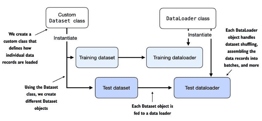
Figure A.10 PyTorch implements a Dataset and a DataLoader class. The Dataset class is used to instantiate objects that define how each data record is loaded. The DataLoader handles how the data is shuffled and assembled into batches.
train_loader = DataLoader(
    dataset=train_ds,
    batch_size=2,
    shuffle=True,
    num_workers=0,      # crucial for parallelizing data loading and preprocessing.
    drop_last=True      # drop the last batch in each epoch(因为最后一个批次的数量可能不够)
)
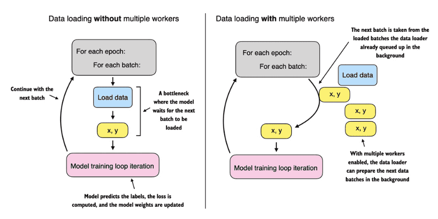
Figure A.11 参数 num_workers 用于控制数据loading的工作线程,当num_workers=0时(像如图左边一样),计算损失值和加载数据一次只能做一个(计算完损失后,gpu会空闲等待数据载入);而 num_workers 启动后,载入数据和计算损失值可以并发执行(像如图右边一样)。Loading data without multiple workers (setting num_workers=0) will create a data loading bottleneck where the model sits idle until the next batch is loaded as illustrated in the left subpanel. If multiple workers are enabled, the data loader can already queue up the next batch in the background as shown in the right subpanel.
警告
or Jupyter notebooks, setting num_workers to greater than 0 can sometimes lead to issues related to the sharing of resources between different processes, resulting in errors or notebook crashes.
备注
根据经验,设置 num_workers=4 通常会在许多实际数据集上带来最佳性能,但最佳设置取决于您的硬件以及用于加载 Dataset 类中定义的训练示例的代码。
A.7 A typical training loop
Listing A.9 Neural network training in PyTorch
import torch.nn.functional as F

torch.manual_seed(123)
model = NeuralNetwork(num_inputs=2, num_outputs=2) #A
optimizer = torch.optim.SGD(model.parameters(), lr=0.5) #B

num_epochs = 3
for epoch in range(num_epochs):
    model.train()
    for batch_idx, (features, labels) in enumerate(train_loader):
        logits = model(features)
        loss = F.cross_entropy(logits, labels)
        optimizer.zero_grad() #C
        loss.backward() #D
        optimizer.step() #E
        ### LOGGING
        print(f"Epoch: {epoch+1:03d}/{num_epochs:03d}"
            f" | Batch {batch_idx:03d}/{len(train_loader):03d}"
            f" | Train Loss: {loss:.2f}")
    model.eval()
    # Optional model evaluation
Listing A.10 A function to compute the prediction accuracy
def compute_accuracy(model, dataloader):
    model = model.eval()
    correct = 0.0
    total_examples = 0
    for idx, (features, labels) in enumerate(dataloader):
        with torch.no_grad():
            logits = model(features)
        predictions = torch.argmax(logits, dim=1)
        compare = labels == predictions #A
        correct += torch.sum(compare) #B
        total_examples += len(compare)
    return (correct / total_examples).item() #C
A.8 Saving and loading models
模型保存:
torch.save(model.state_dict(), "model.pth")

# model.state_dict 是一个 Python 字典对象,它将模型中的每一层映射到其可训练参数(权重和偏差)
模型载入:
model = NeuralNetwork(2, 2)  # 架构需要与原始保存的模型完全匹配
model.load_state_dict(torch.load("model.pth"))
A.9 Optimizing training performance with GPUs
A.9.1 PyTorch computations on GPU devices
CPU:
tensor_1 = torch.tensor([1., 2., 3.])
tensor_2 = torch.tensor([4., 5., 6.])
print(tensor_1 + tensor_2)

# 输出
# tensor([5., 7., 9.])
GPU:
tensor_1 = tensor_1.to("cuda")
tensor_2 = tensor_2.to("cuda")
print(tensor_1 + tensor_2)

# 输出
tensor([5., 7., 9.], device='cuda:0')
A.9.2 Single-GPU training
# Nvidia GPU
device = torch.device("cuda" if torch.cuda.is_available() else "cpu")

# Apple Silicon 芯片
device = torch.device("mps" if torch.backends.mps.is_available() else "cpu")
计算CPU&GPU的计算速度:
# CPU
a = torch.rand(100, 200)
b = torch.rand(200, 300)
%timeit a@b

# GPU
a, b = a.to("cuda"), b.to("cuda")
%timeit a @ b
A.9.3 Training with multiple GPUs
分布式训练是将模型训练划分到多个 GPU 和机器上的概念。
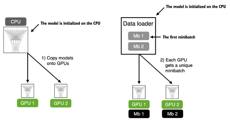
Figure A.12 The model and data transfer in DDP involves two key steps. First, we create a copy of the model on each of the GPUs. Then we divide the input data into unique minibatches that we pass on to each model copy.
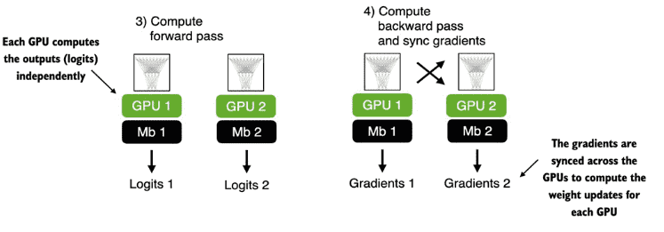
Figure A.13 The forward and backward pass in DDP are executed independently on each GPU with its corresponding data subset. Once the forward and backward passes are completed, gradients from each model replica (on each GPU) are synchronized across all GPUs. This ensures that every model replica has the same updated weights.
备注
DDP does not function properly within interactive Python environments like Jupyter notebooks, which don’t handle multiprocessing in the same way a standalone Python script does.
如果您的机器有四个 GPU 并且您只想使用第一个和第三个 GPU:
CUDA_VISIBLE_DEVICES=0,2 python some_script.py
A.10 Summary
PyTorch is an open-source library that consists of three core components: a
tensor library,automatic differentiation functions, anddeep learning utilities.PyTorch’s tensor library is similar to array libraries like NumPy
In the context of PyTorch, tensors are array-like data structures to represent
scalars,vectors,matrices, andhigher-dimensional arrays. PyTorch tensors can be executed on the CPU, but one major advantage of PyTorch’s tensor format is its GPU support to accelerate computations.The
automatic differentiation (autograd)capabilities in PyTorch allow us to conveniently train neural networks using backpropagation without manually deriving gradients.The deep learning utilities in PyTorch provide building blocks for creating custom deep neural networks.
PyTorch includes
DatasetandDataLoaderclasses to set up efficient data loading pipelines.It’s easiest to train models on a CPU or single GPU.
Using
DistributedDataParallelis the simplest way in PyTorch to accelerate the training if multiple GPUs are available.
Appendix B. References and Further Reading
Chapter 1: Understanding LLM
“Attention Is All You Need” (2017) by Vaswani et al., https://arxiv.org/abs/1706.03762
“BERT: Pre-training of Deep Bidirectional Transformers for Language Understanding” (2018) by Devlin et al., https://arxiv.org/abs/1810.04805
The paper describing the decoder-style GPT-3 model, which inspired modern LLMs and will be used as a template for implementing an LLM from scratch in this book, is “Language Models are Few-Shot Learners” (2020) by Brown et al., https://arxiv.org/abs/2005.14165
The following covers the original vision transformer for classifying images, which illustrates that transformer architectures are not only restricted to text inputs: “An Image is Worth 16x16 Words: Transformers for Image Recognition at Scale” (2020) by Dosovitskiy et al., https://arxiv.org/abs/2010.11929
Meta AI’s model is a popular implementation of a GPT-like model that is openly available in contrast to GPT-3 and ChatGPT: “Llama 2: Open Foundation and Fine-Tuned Chat Models” (2023) by Touvron et al., https://arxiv.org/abs/2307.092881
The following paper provides the reference for InstructGPT for fine-tuning GPT-3: “Training Language Models to Follow Instructions with Human Feedback” (2022) by Ouyang et al., https://arxiv.org/abs/2203.02155
For readers interested in additional details about the dataset references in section 1.5, this paper describes the publicly available The Pile dataset curated by Eleuther AI: “The Pile: An 800GB Dataset of Diverse Text for Language Modeling” (2020) by Gao et al., https://arxiv.org/abs/2101.00027
Chapter 2: Working with Text Data
The code for the byte pair encoding tokenizer used to train GPT- 2 was open-sourced by OpenAI: https://github.com/openai/gpt-2/blob/master/src/encoder.py
OpenAI provides an interactive web UI to illustrate how the byte pair tokenizer in GPT models works: https://platform.openai.com/tokenizer
“A Minimal Implementation of a BPE Tokenizer,” https://github.com/karpathy/minbpe
Chapter 3: Coding Attention Mechanisms
A Minimal Implementation of a BPE Tokenizer,” https://github.com/karpathy/minbpe
The concept of self-attention as scaled dot-product attention was introduced in the original transformer paper: “Attention Is All You Need” (2017) by Vaswani et al., https://arxiv.org/abs/1706.03762
- FlashAttention is a highly efficient implementation of a self- attention mechanism, which accelerates the computation process by optimizing memory access patterns. FlashAttention is mathematically the same as the standard self-attention mechanism but optimizes the computational process for efficiency:
“FlashAttention: Fast and Memory-Efficient Exact Attention with IO-Awareness” (2022) by Dao et al., https://arxiv.org/abs/2205.14135
“FlashAttention-2: Faster Attention with Better Parallelism and Work Partitioning” (2023) by Dao, https://arxiv.org/abs/2307.08691
“Dropout: A Simple Way to Prevent Neural Networks from Overfitting” (2014) by Srivastava et al., https://jmlr.org/papers/v15/srivastava14a.html
Chapter 4: Implementing a GPT model
“Layer Normalization” (2016) by Ba, Kiros, and Hinton, https://arxiv.org/abs/1607.06450
“On Layer Normalization in the Transformer Architecture” (2020) by Xiong et al., https://arxiv.org/abs/2002.04745
“Gaussian Error Linear Units (GELUs)” (2016) by Hendricks and Gimpel, https://arxiv.org/abs/1606.08415
NanoGPT is a code repository with a minimalist yet efficient implementation of a GPT-2 model, similar to the model implemented in this book. “NanoGPT, a Repository for Training Medium-Sized GPTs, https://github.com/karpathy/nanoGPT
Chapter 5: Pretraining on Unlabeled Data
L8.2 Logistic Regression Loss Function, https://www.youtube.com/watch?v=GxJe0DZvydM
L8.7.1 OneHot Encoding and Multi-category Cross Entropy, https://www.youtube.com/watch?v=4n71-tZ94yk
Understanding Onehot Encoding and Cross Entropy in PyTorch, https://mng.bz/o05v
- The following two papers detail the dataset, hyperparameter, and architecture details used for pretraining LLMs:
“Pythia: A Suite for Analyzing Large Language Models Across Training and Scaling” (2023) by Biderman et al., https://arxiv.org/abs/2304.01373
“OLMo: Accelerating the Science of Language Models” (2024) by Groeneveld et al., https://arxiv.org/abs/2402.00838
The paper that originally introduced top-k sampling is “Hierarchical Neural Story Generation” (2018) by Fan et al., https://arxiv.org/abs/1805.04833
Top-p sampling, https://en.wikipedia.org/wiki/Top-p_sampling
“Diverse Beam Search: Decoding Diverse Solutions from Neural Sequence Models” (2016) by Vijayakumar et al., https://arxiv.org/abs/1610.02424
Chapter 6: Fine-tuning for classification
- different types of fine- tuning are
“Using and Finetuning Pretrained Transformers,” https://mng.bz/VxJG
“Finetuning Large Language Models,” https://mng.bz/x28X
Additional spam classification experiments(fine-tuning the first output token versus the last output token), https://mng.bz/AdJx
Chapter 7: Fine-tuning to follow instructions
- datasets for instruction fine-tuning:
“Stanford Alpaca: An Instruction-Following Llama Model,” https://github.com/tatsu-lab/stanford_alpaca
- Preference fine-tuning is an optional step after instruction fine- tuning to align the LLM more closely with human preferences. The following articles by the author provide more information about this process:
“LLM Training: RLHF and Its Alternatives,” https://mng.bz/ZVPm
“Tips for LLM Pretraining and Evaluating Reward Models,” https://mng.bz/RNXj
Appendix A: PyTorch
If you want to learn more about model evaluation in machine learning, I recommend my article “Model Evaluation, Model Selection, and Algorithm Selection in Machine Learning” (2018) by Sebastian Raschka, https://arxiv.org/abs/1811.12808
For readers who are interested in a refresher or gentle introduction to calculus, I’ve written a chapter on calculus that is freely available on my website: “Introduction to Calculus,” by Sebastian Raschka, https://mng.bz/WEyW
If you want to learn more about gradient accumulation, please see the following article: “Finetuning Large Language Models on a Single GPU Using Gradient Accumulation” by Sebastian Raschka, https://mng.bz/8wPD
DDP, which is a popular approach for training deep learning models across multiple GPUs. “Introducing PyTorch Fully Sharded Data Parallel (FSDP) API,” https://mng.bz/EZJR
Appendix C. Exercise Solutions
ignore
Appendix D. Adding Bells and Whistles to the Training Loop
In this appendix, we enhance the training function for the pretraining and fine-tuning processes covered in chapters 5 to 7.
it covers:
learning rate warmup,
cosine decay,
gradient clipping.
D.1 Learning rate warmup
When training complex models like LLMs, implementing learning rate warmup can help stabilize the training
In learning rate warmup, we gradually increase the learning rate from a very low value (
initial_lr) to a user-specified maximum (peak_lr这个是原本用户指定的学习率)This way, the model will start the training with small weight updates, which helps decrease the risk of large destabilizing updates during the training
n_epochs = 15
initial_lr = 0.0001
peak_lr = 0.01
Typically, the number of warmup steps is between 0.1% to 20% of the total number of steps
We can compute the increment as the difference between the
peak_lrandinitial_lrdivided by the number of warmup steps
total_steps = len(train_loader) * n_epochs
warmup_steps = int(0.2 * total_steps)   # 20% warmup
print(warmup_steps)


lr_increment = (peak_lr - initial_lr) / warmup_steps

global_step = -1
track_lrs = []

optimizer = torch.optim.AdamW(model.parameters(), weight_decay=0.1)

for epoch in range(n_epochs):
    for input_batch, target_batch in train_loader:
        optimizer.zero_grad()
        global_step += 1

        if global_step < warmup_steps:
            lr = initial_lr + global_step * lr_increment
        else:
            lr = peak_lr

        # Apply the calculated learning rate to the optimizer
        for param_group in optimizer.param_groups:
            param_group["lr"] = lr
        track_lrs.append(optimizer.param_groups[0]["lr"])

        # Calculate loss and update weights
        # ...
D.2 Cosine decay
Another popular technique for training complex deep neural networks is
cosine decay, which also adjusts the learning rate across training epochsIn cosine decay, the learning rate follows a
cosine curve, decreasing from its initial value to near zero following a half-cosine cycleThis gradual reduction is designed to slow the pace of learning as the model begins to improve its weights; it reduces the risk of overshooting minima as the training progresses, which is crucial for stabilizing the training in its later stages
Cosine decay is often preferred over linear decay for its smoother transition in learning rate adjustments, but linear decay is also used in practice (for example, [OLMo: Accelerating the Science of Language Models](https://arxiv.org/abs/2402.00838))
import math

min_lr = 0.1 * initial_lr
track_lrs = []

lr_increment = (peak_lr - initial_lr) / warmup_steps
total_training_steps = len(train_loader) * n_epochs

global_step = -1

for epoch in range(n_epochs):
    for input_batch, target_batch in train_loader:
        optimizer.zero_grad()
        global_step += 1

        # Adjust the learning rate based on the current phase (warmup or cosine annealing)
        if global_step < warmup_steps:
            # Linear warmup
            lr = initial_lr + global_step * lr_increment
        else:
            # Cosine annealing after warmup
            progress = ((global_step - warmup_steps) /
                        (total_training_steps - warmup_steps))
            lr = min_lr + (peak_lr - min_lr) * 0.5 * (1 + math.cos(math.pi * progress))

        # Apply the calculated learning rate to the optimizer
        for param_group in optimizer.param_groups:
            param_group["lr"] = lr
        track_lrs.append(optimizer.param_groups[0]["lr"])

        # Calculate loss and update weights
D.3 Gradient clipping
Gradient clipping is yet another technique used to stabilize the training when training LLMs
By setting a threshold, gradients exceeding this limit are scaled down to a maximum magnitude to ensure that the updates to the model’s parameters during backpropagation remain within a manageable range
For instance, using the
max_norm=1.0setting in PyTorch’sclip_grad_norm_method means that the norm of the gradients is clipped such that their maximum norm does not exceed 1.0the “norm” refers to a measure of the gradient vector’s length (or magnitude) in the parameter space of the model
Specifically, it’s the L2 norm, also known as the Euclidean norm
Mathematically, for a vector \(\mathbf{v}\) with components \(\mathbf{v} = [v_1, v_2, ..., v_n]\)
the L2 norm is defined as:
The L2 norm is calculated similarly for matrices.
Let’s assume our gradient matrix is:
And we want to clip these gradients with a max_norm of 1.
First, we calculate the L2 norm of these gradients:
Since \(\|G\|_2 = 5\) is greater than our
max_normof 1, we need to scale down the gradients so that their norm is exactly 1. The scaling factor is calculated as \(\frac{max\_norm}{\|G\|_2} = \frac{1}{5}\) .Therefore, the scaled gradient matrix
G'will be as follows:
If we call .backward(), PyTorch will calculate the gradients and store them in a .grad attribute for each weight (parameter) matrix:
loss = calc_loss_batch(input_batch, target_batch, model, device)
loss.backward()
Let’s define a utility function to calculate the highest gradient based on all model weights
def find_highest_gradient(model):
    max_grad = None
    for param in model.parameters():
        if param.grad is not None:
            grad_values = param.grad.data.flatten()
            max_grad_param = grad_values.max()
            if max_grad is None or max_grad_param > max_grad:
                max_grad = max_grad_param
    return max_grad

print(find_highest_gradient(model))
# 输出
# tensor(0.0411)
Applying gradient clipping, we can see that the largest gradient is now substantially smaller:
torch.nn.utils.clip_grad_norm_(model.parameters(), max_norm=1.0)
print(find_highest_gradient(model))
# 输出
# tensor(0.0185)
D.4 The modified training function
Now let’s add the three concepts covered above (
learning rate warmup,cosine decay, and gradient clipping) to the train_model_simple function covered in chapter 5 to create the more sophisticated train_model function below:
from previous_chapters import evaluate_model, generate_and_print_sample

BOOK_VERSION = True


def train_model(model, train_loader, val_loader, optimizer, device,
                n_epochs, eval_freq, eval_iter, start_context, tokenizer,
                warmup_steps, initial_lr=3e-05, min_lr=1e-6):

    train_losses, val_losses, track_tokens_seen, track_lrs = [], [], [], []
    tokens_seen, global_step = 0, -1

    # Retrieve the maximum learning rate from the optimizer
    peak_lr = optimizer.param_groups[0]["lr"]

    # Calculate the total number of iterations in the training process
    total_training_steps = len(train_loader) * n_epochs

    # Calculate the learning rate increment during the warmup phase
    lr_increment = (peak_lr - initial_lr) / warmup_steps

    for epoch in range(n_epochs):
        model.train()
        for input_batch, target_batch in train_loader:
            optimizer.zero_grad()
            global_step += 1

            # Adjust the learning rate based on the current phase (warmup or cosine annealing)
            if global_step < warmup_steps:
                # Linear warmup
                lr = initial_lr + global_step * lr_increment
            else:
                # Cosine annealing after warmup
                progress = ((global_step - warmup_steps) /
                            (total_training_steps - warmup_steps))
                lr = min_lr + (peak_lr - min_lr) * 0.5 * (1 + math.cos(math.pi * progress))

            # Apply the calculated learning rate to the optimizer
            for param_group in optimizer.param_groups:
                param_group["lr"] = lr
            track_lrs.append(lr)  # Store the current learning rate

            # Calculate and backpropagate the loss
            loss = calc_loss_batch(input_batch, target_batch, model, device)
            loss.backward()

            # Apply gradient clipping after the warmup phase to avoid exploding gradients

            if BOOK_VERSION:
                if global_step > warmup_steps:
                    torch.nn.utils.clip_grad_norm_(model.parameters(), max_norm=1.0)
            else:
                if global_step >= warmup_steps:  # the book originally used global_step > warmup_steps, which lead to a skipped clipping step after warmup
                    torch.nn.utils.clip_grad_norm_(model.parameters(), max_norm=1.0)

            optimizer.step()
            tokens_seen += input_batch.numel()

            # Periodically evaluate the model on the training and validation sets
            if global_step % eval_freq == 0:
                train_loss, val_loss = evaluate_model(
                    model, train_loader, val_loader,
                    device, eval_iter
                )
                train_losses.append(train_loss)
                val_losses.append(val_loss)
                track_tokens_seen.append(tokens_seen)
                # Print the current losses
                print(f"Ep {epoch+1} (Iter {global_step:06d}): "
                      f"Train loss {train_loss:.3f}, "
                      f"Val loss {val_loss:.3f}"
                )

        # Generate and print a sample from the model to monitor progress
        generate_and_print_sample(
            model, tokenizer, device, start_context
        )

    return train_losses, val_losses, track_tokens_seen, track_lrs
使用:
peak_lr = 0.001  # this was originally set to 5e-4 in the book by mistake
optimizer = torch.optim.AdamW(model.parameters(), lr=peak_lr, weight_decay=0.1)  # the book accidentally omitted the lr assignment

train_losses, val_losses, tokens_seen, lrs = train_model(
    model, train_loader, val_loader, optimizer, device, n_epochs=n_epochs,
    eval_freq=5, eval_iter=1, start_context="Every effort moves you",
    tokenizer=tokenizer, warmup_steps=warmup_steps,
    initial_lr=1e-5, min_lr=1e-5
)
# 输出
Ep 1 (Iter 000000): Train loss 10.934, Val loss 10.939
Ep 1 (Iter 000005): Train loss 9.151, Val loss 9.461
...
Ep 14 (Iter 000120): Train loss 0.038, Val loss 6.907
Ep 14 (Iter 000125): Train loss 0.040, Val loss 6.912
Ep 15 (Iter 000130): Train loss 0.041, Val loss 6.915
appendix E Parameter-efficient fine- tuning with LoRA
Low-rank adaptation (LoRA) is one of the most widely used techniques for parameter-efficient fine-tuning.
E.1 Introduction to LoRA
LoRA is a technique that adapts a pretrained model to better suit a specific, often smaller dataset by adjusting only a small subset of the model’s weight parameters.
The LoRA method is useful and popular because it enables efficient fine-tuning of large models on task-specific data, significantly cutting down on the computational costs and resources usually required for fine-tuning.
Suppose we have a large weight matrix
Wfor a given layerDuring backpropagation, we learn a \(\Delta W\) matrix, which contains information on how much we want to update the original weights to minimize the loss function during training
In regular training and finetuning, the weight update is defined as follows:
The LoRA method offers a more efficient alternative to computing the weight updates \(\Delta W\) by learning an approximation of it, \(\Delta W \approx AB\).
In other words, in LoRA, we have the following, where
AandBare two small weight matrices:
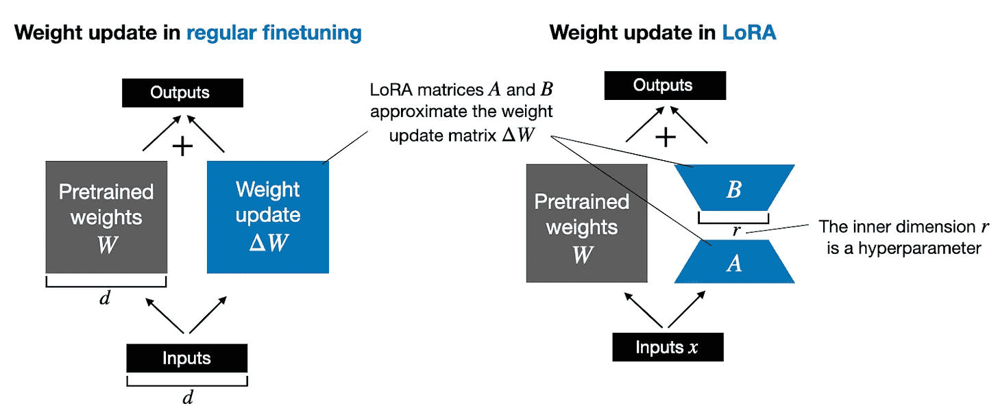
Figure E.1 A comparison between weight update methods: regular fine-tuning and LoRA. Regular fine-tuning involves updating the pretrained weight matrix W directly with DW (left). LoRA uses two smaller matrices, A and B, to approximate DW, where the product AB is added to W, and r denotes the inner dimension, a tunable hyperparameter (right).
If you paid close attention, the full finetuning and LoRA depictions in the figure above look slightly different from the formulas I have shown earlier
That’s due to the distributive law of matrix multiplication: we don’t have to add the weights with the updated weights but can keep them separate
For instance, if
xis the input data, then we can write the following for regular finetuning:
The fact that we can keep the LoRA weight matrices separate makes LoRA especially attractive
In practice, this means that we don’t have to modify the weights of the pretrained model at all, as we can apply the LoRA matrices on the fly
E.2 Preparing the dataset
E.3 Initializing the model
像 chapter 6 一样替换 output layer:
num_classes = 2
model.out_head = torch.nn.Linear(in_features=768, out_features=num_classes)
E.4 Parameter-efficient finetuning with LoRA
We begin by initializing a LoRALayer that creates the matrices
AandB, along with thealphascaling hyperparameter and therank(r) hyperparameters
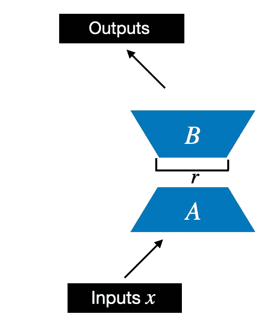
Figure E.2 The LoRA matrices A and B are applied to the layer inputs and are involved in computing the model outputs. The inner dimension r of these matrices serves as a setting that adjusts the number of trainable parameters by varying the sizes of A and B.
import math

class LoRALayer(torch.nn.Module):
    def __init__(self, in_dim, out_dim, rank, alpha):
        super().__init__()
        self.A = torch.nn.Parameter(torch.empty(in_dim, rank))
        torch.nn.init.kaiming_uniform_(self.A, a=math.sqrt(5))  # similar to standard weight initialization
        self.B = torch.nn.Parameter(torch.zeros(rank, out_dim))  # 由于初始时,self.B为0
        self.alpha = alpha

    def forward(self, x):
        x = self.alpha * (x @ self.A @ self.B)
        return x
In the code above,
rankis a hyperparameter that controls the inner dimension of the matricesAandBIn other words, this parameter controls the number of additional parameters introduced by LoRA and is a key factor in determining the balance between model adaptability and parameter efficiency
The second hyperparameter,
alpha, is a scaling hyperparameter applied to the output of the low-rank adaptationIt essentially controls the extent to which the adapted layer’s output is allowed to influence the original output of the layer being adapted
This can be seen as a way to regulate the impact of the low-rank adaptation on the layer’s output
So far, the
LoRALayerclass we implemented above allows us to transform the layer inputsxHowever, in LoRA, we are usually interested in replacing existing
Linearlayers so that the weight update is applied to the existing pretrained weights, as shown in the figure below
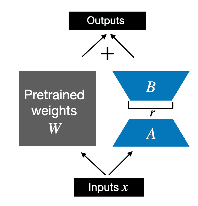
Figure E.3 The integration of LoRA into a model layer. The original pretrained weights (W) of a layer are combined with the outputs from LoRA matrices (A and B), which approximate the weight update matrix (DW). The final output is calculated by adding the output of the adapted layer (using LoRA weights) to the original output.
To incorporate the original
Linearlayer weights as shown in the figure above, we implement aLinearWithLoRAlayer below that uses the previously implemented LoRALayer and can be used to replace existingLinearlayers in a neural network, for example, the self-attention module or feed forward modules in an LLM
class LinearWithLoRA(torch.nn.Module):
    def __init__(self, linear, rank, alpha):
        super().__init__()
        self.linear = linear
        self.lora = LoRALayer(
            linear.in_features, linear.out_features, rank, alpha
        )

    def forward(self, x):
        return self.linear(x) + self.lora(x)
To try LoRA on the GPT model we defined earlier, we define a
replace_linear_with_lorafunction to replace allLinearlayers in the model with the newLinearWithLoRAlayers
def replace_linear_with_lora(model, rank, alpha):
    for name, module in model.named_children():
        if isinstance(module, torch.nn.Linear):
            # Replace the Linear layer with LinearWithLoRA
            setattr(model, name, LinearWithLoRA(module, rank, alpha))
        else:
            # Recursively apply the same function to child modules
            replace_linear_with_lora(module, rank, alpha)
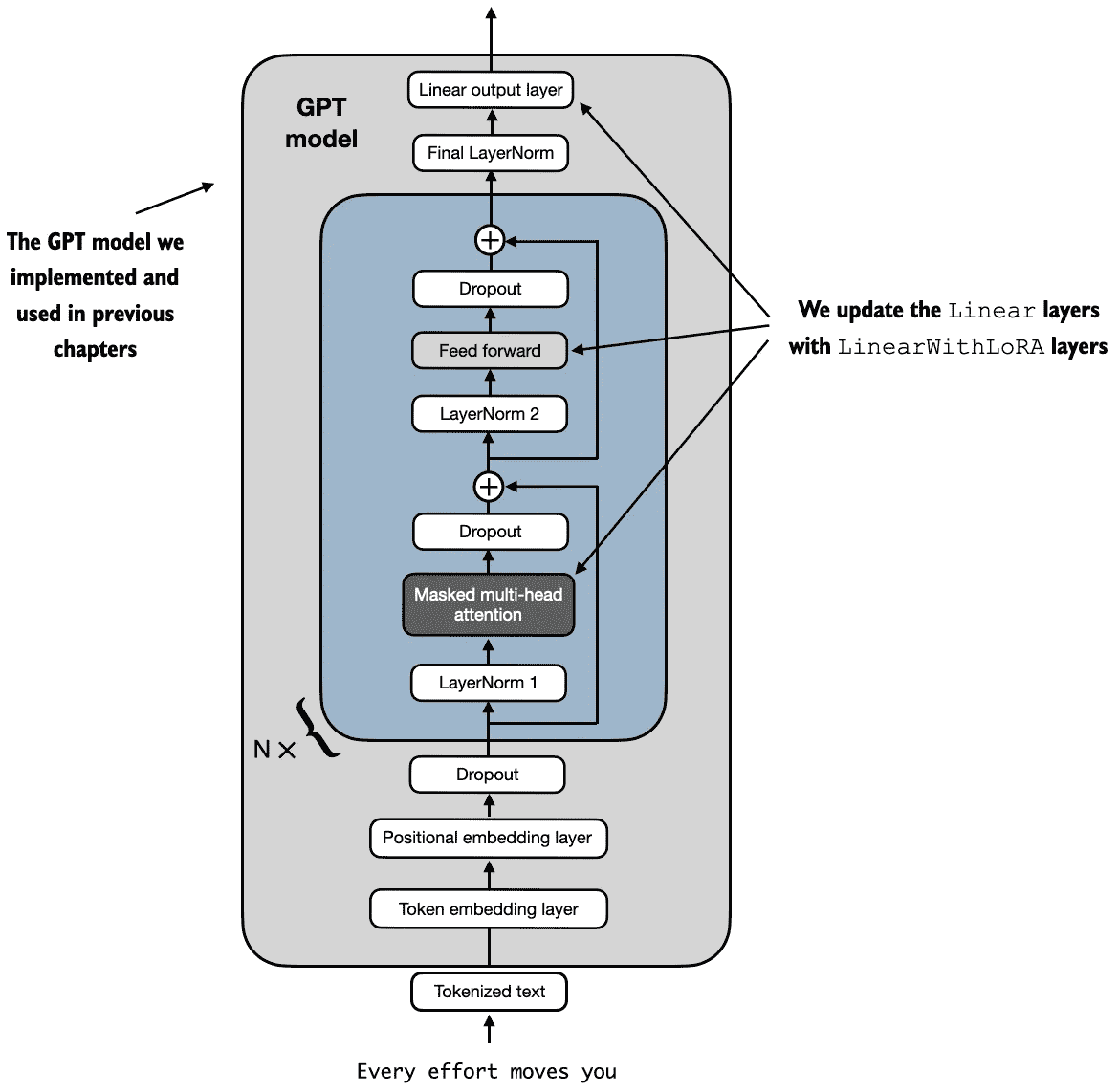
Figure E.4 The architecture of the GPT model. It highlights the parts of the model where Linear layers are upgraded to LinearWithLoRA layers for parameter-efficient fine-tuning.
We then freeze the original model parameter and use the
replace_linear_with_lorato replace the saidLinearlayers using the code belowThis will replace the
Linearlayers in the LLM withLinearWithLoRAlayers
total_params = sum(p.numel() for p in model.parameters() if p.requires_grad)
print(f"Total trainable parameters before: {total_params:,}")

for param in model.parameters():
    param.requires_grad = False

total_params = sum(p.numel() for p in model.parameters() if p.requires_grad)
print(f"Total trainable parameters after: {total_params:,}")
# 输出
# Total trainable parameters before: 124,441,346
# Total trainable parameters after: 0
replace_linear_with_lora(model, rank=16, alpha=16)

total_params = sum(p.numel() for p in model.parameters() if p.requires_grad)
print(f"Total trainable LoRA parameters: {total_params:,}")
# 输出
# Total trainable LoRA parameters: 2,666,528
打印看下现在模型的结构
GPTModel(
  (tok_emb): Embedding(50257, 768)
  (pos_emb): Embedding(1024, 768)
  (drop_emb): Dropout(p=0.0, inplace=False)
  (trf_blocks): Sequential(
    (0): TransformerBlock(
      (att): MultiHeadAttention(
        (W_query): LinearWithLoRA(
          (linear): Linear(in_features=768, out_features=768, bias=True)
          (lora): LoRALayer()
        )
        (W_key): LinearWithLoRA(
          (linear): Linear(in_features=768, out_features=768, bias=True)
          (lora): LoRALayer()
        )
        (W_value): LinearWithLoRA(
          (linear): Linear(in_features=768, out_features=768, bias=True)
          (lora): LoRALayer()
        )
        (out_proj): LinearWithLoRA(
          (linear): Linear(in_features=768, out_features=768, bias=True)
          (lora): LoRALayer()
        )
        (dropout): Dropout(p=0.0, inplace=False)
      )
      (ff): FeedForward(
        (layers): Sequential(
          (0): LinearWithLoRA(
            (linear): Linear(in_features=768, out_features=3072, bias=True)
            (lora): LoRALayer()
          )
          (1): GELU()
          (2): LinearWithLoRA(
            (linear): Linear(in_features=3072, out_features=768, bias=True)
            (lora): LoRALayer()
          )
        )
      )
      (norm1): LayerNorm()
      (norm2): LayerNorm()
      (drop_resid): Dropout(p=0.0, inplace=False)
    )
    ... ... # 省略11个
  )
  (final_norm): LayerNorm()
  (out_head): LinearWithLoRA(
    (linear): Linear(in_features=768, out_features=2, bias=True)
    (lora): LoRALayer()
  )
)
同样的调优步骤:
optimizer = torch.optim.AdamW(model.parameters(), lr=5e-5, weight_decay=0.1)

num_epochs = 5
train_losses, val_losses, train_accs, val_accs, examples_seen = train_classifier_simple(
    model, train_loader, val_loader, optimizer, device,
    num_epochs=num_epochs, eval_freq=50, eval_iter=5,
)
The resulting accuracy values are:
Training accuracy: 100.00%
Validation accuracy: 96.64%
Test accuracy: 98.00%
备注
结论:However, the slightly lower validation and test accuracies (96.64% and 97.33%, respectively) suggest a small degree of overfitting, as the model does not generalize quite as well on unseen data compared to the training set. Overall, the results are very impressive, considering we fine-tuned only a relatively small number of model weights (2.7 million LoRA weights instead of the original 124 million model weights).
其他
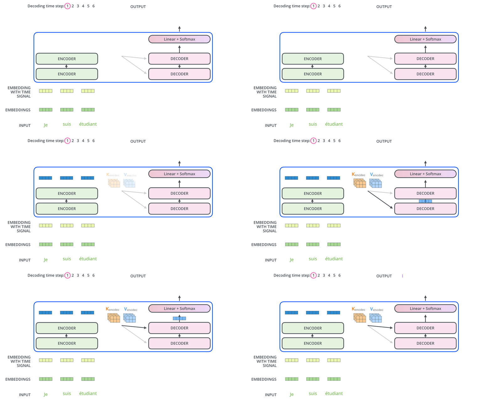
The encoder start by processing the input sequence. The output of the top encoder is then transformed into a set of attention vectors K and V. These are to be used by each decoder in its “encoder-decoder attention” layer which helps the decoder focus on appropriate places in the input sequence:
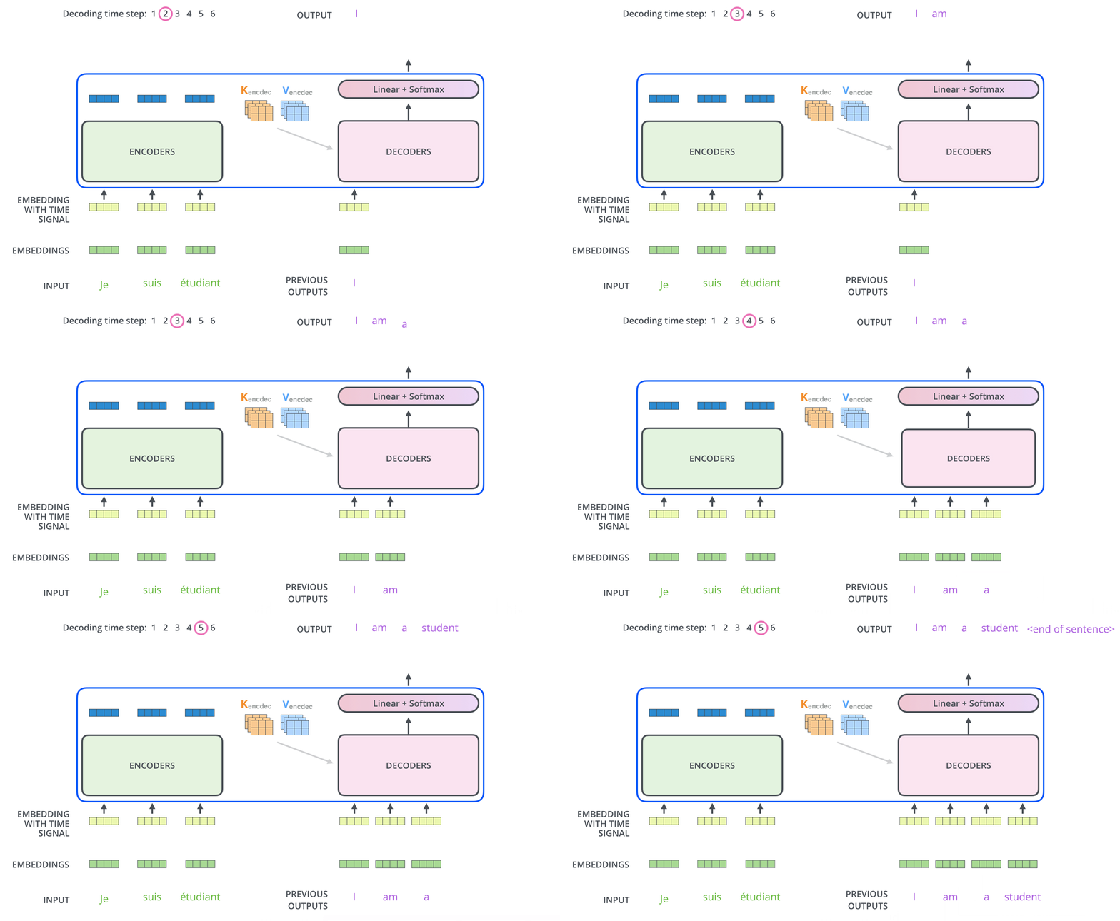
The following steps repeat the process until a special symbol is reached indicating the transformer decoder has completed its output. The output of each step is fed to the bottom decoder in the next time step, and the decoders bubble up their decoding results just like the encoders did. And just like we did with the encoder inputs, we embed and add positional encoding to those decoder inputs to indicate the position of each word.
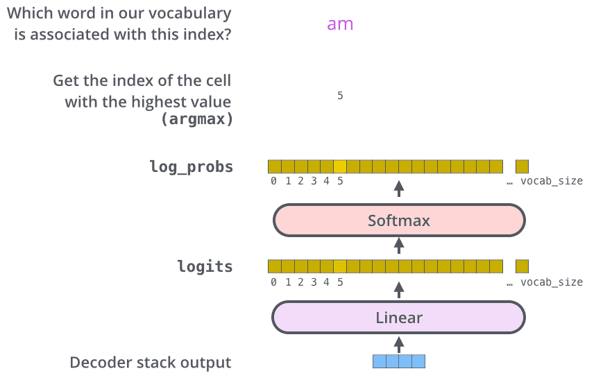
The Linear layer is a simple fully connected neural network that projects the vector produced by the stack of decoders, into a much, much larger vector called a logits vector. The softmax layer then turns those scores into probabilities (all positive, all add up to 1.0). The cell with the highest probability is chosen, and the word associated with it is produced as the output for this time step.