Kaggle Learn
Intermediate Machine Learning
Missing Values
There are many ways data can end up with missing values. For example:
A 2 bedroom house won't include a value for the size of a third bedroom.
A survey respondent may choose not to share his income.
Most machine learning libraries (including scikit-learn) give an error if you try to build a model using data with missing values. So you’ll need to choose one of the strategies below.
Three Approaches
1) A Simple Option: Drop Columns with Missing Values

Unless most values in the dropped columns are missing, the model loses access to a lot of (potentially useful!) information with this approach.
2) A Better Option: Imputation

Imputation fills in the missing values with some number. For instance, we can fill in the mean value along each column.
The imputed value won’t be exactly right in most cases, but it usually leads to more accurate models than you would get from dropping the column entirely.
备注
why did imputation perform better than dropping the columns? The training data has 10864 rows and 12 columns, where three columns contain missing data. For each column, less than half of the entries are missing. Thus, dropping the columns removes a lot of useful information, and so it makes sense that imputation would perform better.
备注
Given that there are so few missing values in the dataset, we’d expect imputation to perform better than dropping columns entirely. However, we see that dropping columns performs slightly better! While this can probably partially be attributed to noise in the dataset, another potential explanation is that the imputation method is not a great match to this dataset. That is, maybe instead of filling in the mean value, it makes more sense to set every missing value to a value of 0, to fill in the most frequently encountered value, or to use some other method.
3) An Extension To Imputation
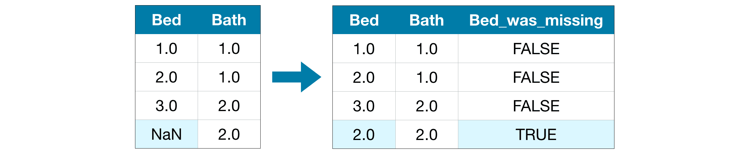
In this approach, we impute the missing values, as before. And, additionally, for each column with missing entries in the original dataset, we add a new column that shows the location of the imputed entries.
Imputation is the standard approach, and it usually works well. However, imputed values may be systematically above or below their actual values (which weren’t collected in the dataset). Or rows with missing values may be unique in some other way. In that case, your model would make better predictions by considering which values were originally missing.
Categorical Variables
A categorical variable takes only a limited number of values.
Consider a survey that asks how often you eat breakfast and provides four options: “Never”, “Rarely”, “Most days”, or “Every day”. In this case, the data is categorical, because responses fall into a fixed set of categories.
If people responded to a survey about which what brand of car they owned, the responses would fall into categories like “Honda”, “Toyota”, and “Ford”. In this case, the data is also categorical.
Three Approaches
1) Drop Categorical Variables
The easiest approach to dealing with categorical variables is to simply remove them from the dataset. This approach will only work well if the columns did not contain useful information.
2) Ordinal Encoding

Ordinal encoding assigns each unique value to a different integer.
This approach assumes an ordering of the categories: “Never” (0) < “Rarely” (1) < “Most days” (2) < “Every day” (3).
This assumption makes sense in this example, because there is an indisputable ranking to the categories. Not all categorical variables have a clear ordering in the values, but we refer to those that do as ordinal variables. For tree-based models (like decision trees and random forests), you can expect ordinal encoding to work well with ordinal variables.
OrdinalEncoder 是 scikit-learn 库中的一个预处理工具,用于将分类特征转换为整数编码。它主要用于处理具有有序类别的特征,即特征的分类值具有一定的顺序关系。
3) One-Hot Encoding
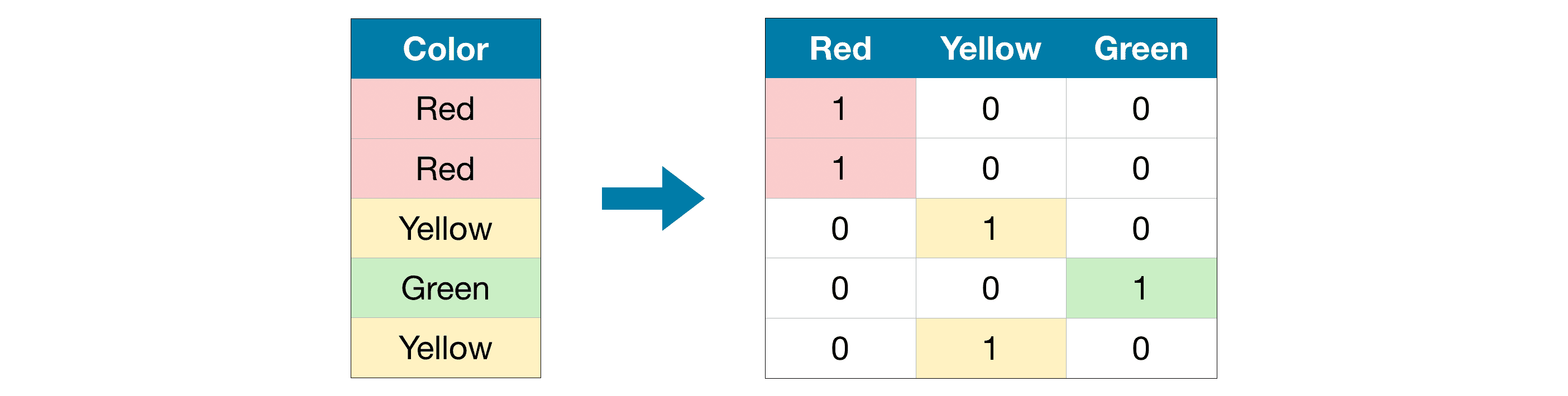
One-hot encoding creates new columns indicating the presence (or absence) of each possible value in the original data.
In the original dataset, “Color” is a categorical variable with three categories: “Red”, “Yellow”, and “Green”. The corresponding one-hot encoding contains one column for each possible value, and one row for each row in the original dataset. Wherever the original value was “Red”, we put a 1 in the “Red” column; if the original value was “Yellow”, we put a 1 in the “Yellow” column, and so on.
In contrast to ordinal encoding, one-hot encoding does not assume an ordering of the categories. Thus, you can expect this approach to work particularly well if there is no clear ordering in the categorical data (e.g., “Red” is neither more nor less than “Yellow”). We refer to categorical variables without an intrinsic ranking as nominal variables.
One-hot encoding generally does not perform well if the categorical variable takes on a large number of values (i.e., you generally won’t use it for variables taking more than 15 different values).
OneHotEncoder 是 scikit-learn 库中的一个预处理工具,用于将分类特征转换为独热编码(One-Hot Encoding)。它将每个分类特征的每个类别转换为一个新的特征,并使用 0 和 1 来表示是否存在该类别。
备注
In general, one-hot encoding (Approach 3) will typically perform best, and dropping the categorical columns (Approach 1) typically performs worst, but it varies on a case-by-case basis.
Pipelines
Pipelines are a simple way to keep your data preprocessing and modeling code organized. Specifically, a pipeline bundles preprocessing and modeling steps so you can use the whole bundle as if it were a single step.
Many data scientists hack together models without pipelines, but pipelines have some important benefits. Those include:
1. Cleaner Code: Accounting for data at each step of preprocessing can get messy.
2. Fewer Bugs: There are fewer opportunities to misapply a step or forget a preprocessing step.
3. Easier to Productionize: pipelines can help to transition a model from a prototype to something deployable at scale.
4. More Options for Model Validation:
示例:
# Preprocessing for numerical data
numerical_transformer = SimpleImputer(strategy='constant')

# Preprocessing for categorical data
categorical_transformer = Pipeline(steps=[
    ('imputer', SimpleImputer(strategy='most_frequent')),
    ('onehot', OneHotEncoder(handle_unknown='ignore'))
])

# Bundle preprocessing for numerical and categorical data
preprocessor = ColumnTransformer(
    transformers=[
        ('num', numerical_transformer, numerical_cols),
        ('cat', categorical_transformer, categorical_cols)
    ])
Cross-Validation
Introduction
Machine learning is an iterative process.
You will face choices about what predictive variables to use, what types of models to use, what arguments to supply to those models, etc. So far, you have made these choices in a data-driven way by measuring model quality with a validation (or holdout) set.
But there are some drawbacks to this approach. To see this, imagine you have a dataset with 5000 rows. You will typically keep about 20% of the data as a validation dataset, or 1000 rows. But this leaves some random chance in determining model scores. That is, a model might do well on one set of 1000 rows, even if it would be inaccurate on a different 1000 rows.
At an extreme, you could imagine having only 1 row of data in the validation set. If you compare alternative models, which one makes the best predictions on a single data point will be mostly a matter of luck!
In general, the larger the validation set, the less randomness (aka “noise”) there is in our measure of model quality, and the more reliable it will be. Unfortunately, we can only get a large validation set by removing rows from our training data, and smaller training datasets mean worse models!
What is cross-validation?
In cross-validation, we run our modeling process on different subsets of the data to get multiple measures of model quality.
For example, we could begin by dividing the data into 5 pieces, each 20% of the full dataset. In this case, we say that we have broken the data into 5 “folds”.
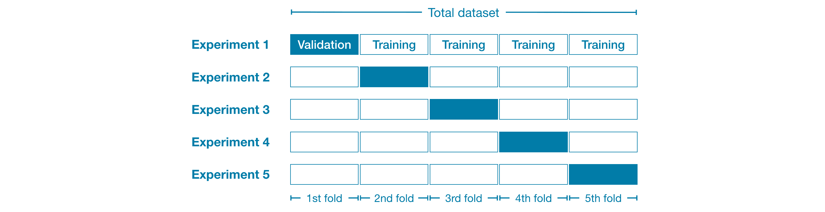
Then, we run one experiment for each fold:
In Experiment 1, we use the first fold as a validation (or holdout) set and everything else as training data. This gives us a measure of model quality based on a 20% holdout set.
In Experiment 2, we hold out data from the second fold (and use everything except the second fold for training the model). The holdout set is then used to get a second estimate of model quality.
We repeat this process, using every fold once as the holdout set. Putting this together, 100% of the data is used as holdout at some point, and we end up with a measure of model quality that is based on all of the rows in the dataset (even if we don’t use all rows simultaneously).
When should you use cross-validation?
Cross-validation gives a more accurate measure of model quality, which is especially important if you are making a lot of modeling decisions. However, it can take longer to run, because it estimates multiple models (one for each fold).
So, given these tradeoffs, when should you use each approach?
For small datasets, where extra computational burden isn’t a big deal, you should run cross-validation.
For larger datasets, a single validation set is sufficient. Your code will run faster, and you may have enough data that there’s little need to re-use some of it for holdout.
There’s no simple threshold for what constitutes a large vs. small dataset. But if your model takes a couple minutes or less to run, it’s probably worth switching to cross-validation.
Alternatively, you can run cross-validation and see if the scores for each experiment seem close. If each experiment yields the same results, a single validation set is probably sufficient.
XGBoost
In this tutorial, you will learn how to build and optimize models with gradient boosting. This method dominates many Kaggle competitions and achieves state-of-the-art results on a variety of datasets.
XGBoost: extreme gradient boosting(极端梯度提升)
Introduction
For much of this course, you have made predictions with the random forest method, which achieves better performance than a single decision tree simply by averaging the predictions of many decision trees.
We refer to the random forest method as an “ensemble method”. By definition, ensemble methods combine the predictions of several models (e.g., several trees, in the case of random forests).
Next, we’ll learn about another ensemble method called gradient boosting.
Gradient Boosting
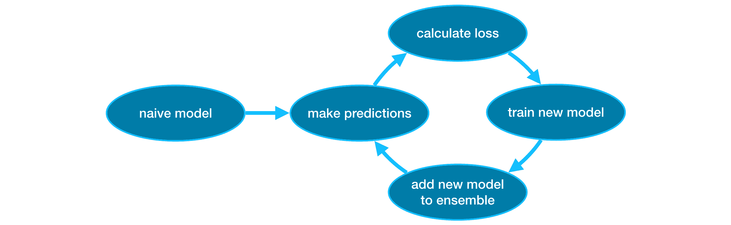
Gradient boosting is a method that goes through cycles to iteratively add models into an ensemble.
It begins by initializing the ensemble with a single model, whose predictions can be pretty naive. (Even if its predictions are wildly inaccurate, subsequent additions to the ensemble will address those errors.)
Then, we start the cycle:
First, we use the current ensemble to generate predictions for each observation in the dataset.
    To make a prediction, we add the predictions from all models in the ensemble.
These predictions are used to calculate a loss function (like mean squared error, for instance).
Then, we use the loss function to fit a new model that will be added to the ensemble.
    Specifically, we determine model parameters so that adding this new model to the ensemble will reduce the loss.
    (Side note:
        The "gradient" in "gradient boosting" refers to the fact that we'll use gradient descent on the loss function
        to determine the parameters in this new model.)
Finally, we add the new model to ensemble, and ...
... repeat!
Data Leakage
Introduction
Data leakage (or leakage) happens when your training data contains information about the target, but similar data will not be available when the model is used for prediction. This leads to high performance on the training set (and possibly even the validation data), but the model will perform poorly in production.
In other words, leakage causes a model to look accurate until you start making decisions with the model, and then the model becomes very inaccurate.
There are two main types of leakage: target leakage and train-test contamination.
Target leakage
Target leakage occurs when your predictors include data that will not be available at the time you make predictions. It is important to think about target leakage in terms of the timing or chronological order that data becomes available, not merely whether a feature helps make good predictions.
目标泄露(Target Leakage)是指在建模过程中,模型能够访问的与目标变量相关的信息泄露到训练数据中。这种泄露可能会导致模型在实际应用中表现良好,但在真实环境下却无法达到预期水平。目标泄露的常见形式包括使用未来数据、将测试数据中的特征信息用于训练、错误地排除可能导致目标变量的特征等。
Example-Imagine you want to predict who will get sick with pneumonia:
got_pneumonia |
age weight |
male |
took_antibiotic_medicine |
… |
|---|---|---|---|---|
False |
65 |
100 False |
False |
… |
False |
72 |
130 True |
False |
… |
True |
58 |
100 False |
True |
… |
People take antibiotic medicines after getting pneumonia in order to recover. The raw data shows a strong relationship between those columns, but took_antibiotic_medicine is frequently changed after the value for got_pneumonia is determined. This is target leakage.
The model would see that anyone who has a value of False for took_antibiotic_medicine didn’t have pneumonia. Since validation data comes from the same source as training data, the pattern will repeat itself in validation, and the model will have great validation (or cross-validation) scores.
But the model will be very inaccurate when subsequently deployed in the real world, because even patients who will get pneumonia won’t have received antibiotics yet when we need to make predictions about their future health.
To prevent this type of data leakage, any variable updated (or created) after the target value is realized should be excluded.
Train-Test Contamination
A different type of leak occurs when you aren’t careful to distinguish training data from validation data.
Recall that validation is meant to be a measure of how the model does on data that it hasn’t considered before. You can corrupt this process in subtle ways if the validation data affects the preprocessing behavior. This is sometimes called train-test contamination.
训练 - 测试污染(Train-Test Contamination)是指在建模过程中,训练数据中的信息无意间或有意地泄漏到测试数据中,从而使测试数据的表现不再真实反映模型对未知数据的泛化能力。这种污染可能会导致模型在测试阶段表现良好,但在真实场景中无法正确泛化。训练 - 测试污染的常见形式包括在数据预处理过程中未正确分离训练和测试数据、使用交叉验证时未正确处理数据的泄漏等。
For example, imagine you run preprocessing (like fitting an imputer for missing values) before calling train_test_split(). The end result? Your model may get good validation scores, giving you great confidence in it, but perform poorly when you deploy it to make decisions.
After all, you incorporated data from the validation or test data into how you make predictions, so the may do well on that particular data even if it can’t generalize to new data. This problem becomes even more subtle (and more dangerous) when you do more complex feature engineering.
If your validation is based on a simple train-test split, exclude the validation data from any type of fitting, including the fitting of preprocessing steps. This is easier if you use scikit-learn pipelines. When using cross-validation, it’s even more critical that you do your preprocessing inside the pipeline!